CS229a - Week 1

Written by hackerwins on June 04, 2019

Introduction

What is Machine Learning?

E = the experience of playing many games of checkers
T = the task of playing checkers
P = the probability that the program will win the next game

In general, any machine learning problem can be assigned to one of two broad classifications: Supervised learning and Unsupervised learning.

Supervised Learning

Regression problem: 연속적인 값을 예측
Classification problem: 이산 적인 값으로 구분(Boolean, Integer)
Support Vector Machine: handle large feature space

Unsupervised Learning

Clustering: i.g. 구글 뉴스, 컴퓨터 클러스터 구성, 사회 관계망 분석
Cocktail party problem: 두 사람의 목소리 분리하기 혹은 노이즈 제거하기

Linear regression with one variable

Model and Cost function

Input: $x_i$
Output: $y_i$
Training set: $(x_i, y_i); i = 1 ...m$
Hypothesis: $h_\theta(x) = \theta_0 + \theta_1x$

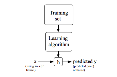
To describe the supervised learning problem slightly more formally, our goal is, given a training set, to learn a function h : X → Y so that h(x) is a “good” predictor for the corresponding value of y. For historical reasons, this function h is called a hypothesis.

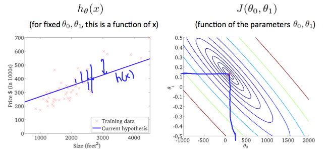
Cost Function, “Squared error function” or “Mean squared error”: this is a function of theta

\[J(\theta_0,\theta_1) =\frac{1}{2m}\sum_{i=1}^m(h_\theta(x_i)-y_i)^2\] \[h_\theta(x_i) = \theta_0 + \theta_1x_i\]

실제 값과 예측 값의 차이의 평균의 최소값
m = number of training example
hypothesis function = prediction
y = real value
우리가 찾아야하는 값: $min J(\theta_0,\theta_1)$

Gradient descent algorithm

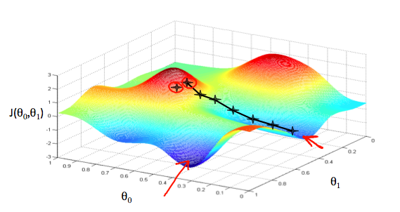
초기 지점에서 기울기를 따라서 작은 값을 찾아 내려감

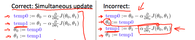
각 스텝 마다 동시에 업데이트 해야 함

repeat until convergence(simultaneously update $j = 0: j = 1$):

\[\theta_j := \theta_j - \alpha\frac{\partial}{\partial\theta_j}J(\theta_0,\theta_1)\]

$:=$: assignment operator
$\alpha$: learning rate, how big a step we take downhill
Derivative term: direction
- partial derivative($$\partialj$): 특정 함수에서 한 가지 변수만 미분하고 나머지는 상수처럼 취급
- tangent: 기울기 값
- derivative term의 값이 양수이면 각 스텝마다 좌측으로 이동
- derivative term의 값이 음수이면 각 스텝마다 우측으로 이동
- learning rate가 너무 작으면, GD가 느려지고 learning rate가 너무 크면 심지어 diverge 된다.
- local minimum에 가까워질 수록 이동하는 거리가 작아짐(기울기가 완만해 지므로)

Gradient descent for Linear regression

repeat until convergence(simultaneously update j = 0 and j = 1):

\[\theta_j := \theta_j - \alpha\frac{\partial}{\partial\theta_j}J(\theta_0,\theta_1)\]

Linear regression model

\[J(\theta_0,\theta_1) =\frac{1}{2m}\sum_{i=1}^m(h_\theta(x_i)-y_i)^2 \\ h_\theta(x_i) = \theta_0 + \theta_1x_i\]

Plugging in the definition of the cost function into derivative term

\[\frac{\theta}{\partial\theta_j}\frac{1}{2m}\sum_{i=1}^m(h_\theta(x_i)-y_i)^2\]

Plugging in the definition of hypothesis

\[\frac{\theta}{\partial\theta_j}\frac{1}{2m}\sum_{i=1}^m(\theta_0 + \theta_1x_i-y_i)^2\]

Calculate partial derivative

\[\theta_i := \theta_i - \alpha\frac{1}{m}\sum_{i=1}^{m}(h_\theta(x^{(i)})-y^{(i)})x^{(i)}\]

Linear regression의 Cost function

Convex function
local optima가 없음, 한 개의 global optima만 존재

Batch Gradient Descent

다수의 training examples의 각각의 GD를 뜻함
ML 사람들이 만든 Batch라는 이름은 좋은 이름이 아니라 생각함 by Andrew Ng

Linear algebra review

Matrices

The dimension of the matrix is going to be written as the number of row times the number of columns in the matrix.

\[A =\begin{bmatrix} 1 & 2 & 3 \\ 4 & 5 & 6 \end{bmatrix}\]

This is a 2 by 3 matrix
$A_{ij}$: “i, j entry” in the ith row, jth column
주로 대문자로 표기함

Vectors

Vector is a matrix that has only 1 column.

\[y =\begin{bmatrix} 1 \\ 4 \\ 5 \end{bmatrix}\]

y is a 3-dimensional vector.
$y_i$: ith element
1-indexed vector: index가 1부터 시작하는 vector, 수학에서 주로 사용함
0-indexed vector: index가 0부터 시작하는 vector, 프로그램에서 주로 사용함
주로 소문자로 표기함

Matrix Addition

\[\begin{bmatrix} 1 & 2 & 3 \\ 4 & 5 & 6 \end{bmatrix} + \begin{bmatrix} 1 & 2 & 3 \\ 4 & 5 & 6 \end{bmatrix} = \begin{bmatrix} 2 & 4 & 6 \\ 8 & 10 & 12 \end{bmatrix}\]

Scalar Multiplication

\[3 \times \begin{bmatrix} 1 & 2 & 3 \\ 4 & 5 & 6 \end{bmatrix} = \begin{bmatrix} 3 & 6 & 9 \\ 12 & 15 & 18 \end{bmatrix}\]

Matrix Vector Multiplication

\[\begin{bmatrix} 1 & 2 \\ 3 & 4 \\ 5 & 6 \end{bmatrix} \times \begin{bmatrix} 1 \\ 2 \end{bmatrix} = \begin{bmatrix} 5 \\ 11 \\ 17 \end{bmatrix}\]

The result of multiplying 3 by 2 matrix with 2 by 1 vector is 3 by 1 matrix(or vector).

Matrix Vector Multiplication을 Linear regression에 사용하면 아래와 같음

House sizes: 2014, 1416, 1534, 852
Hypothesis: $h_\theta(x) = -40 + 0.25x$ $\begin{bmatrix} 1 & 2104 \\ 1 & 1416 \\ 1 & 1534 \\ 1 & 852 \end{bmatrix} \times \begin{bmatrix} -40 \\ 0.25 \end{bmatrix}$

Matrix Matrix Multiplication

\[\begin{bmatrix} 1 & 2 & 3 \\ 4 & 5 & 6 \end{bmatrix} \times \begin{bmatrix} 1 & 2 \\ 3 & 4 \\ 5 & 6 \end{bmatrix} = \begin{bmatrix} 22 & 28 \\ 49 & 64 \end{bmatrix}\]

The result of multiplying 2 by 3 matrix with 3 by 2 matrix is 2 by 2 matrix.

Matrix Vector Multiplication을 Linear regression에 사용하면 아래와 같음

House sizes: 2014, 1416, 1534, 852
3 competing hypothesis:
\[h_\theta(x) = -40 + 0.25x\] \[h_\theta(x) = 200 + 0.1x\] \[h_\theta(x) = -150 + 0.4x\] \[\begin{bmatrix} 1 & 2104 \\ 1 & 1416 \\ 1 & 1534 \\ 1 & 852 \end{bmatrix} \times \begin{bmatrix} -40 & 200 & -150 \\ 0.25 & 0.1 & 0.4\end{bmatrix} = \begin{bmatrix} 486 & 410 & 692 \\ 314 & 342 & 416 \\ 344 & 353 & 464 \\ 173 & 285 & 191 \end{bmatrix}\]

더 살펴보기

Matrix Multiplication properties

Commutative property, 교환법칙: X, not commutative
Associative property, 결합법칙: O

Identity Matrix

Denoted I (or $I_n \times n$)

\[\begin{bmatrix} 1 \end{bmatrix}, \begin{bmatrix} 1 & 0 \\ 0 & 1 \end{bmatrix}, \begin{bmatrix} 1 & 0 & 0 \\ 0 & 1 & 0 \\ 0 & 0 & 1\end{bmatrix} ...\]

: $A \cdot I = I \cdot A = A$

Matrix Inverse and Transpose

Inverse

Identity: $3 \times 3^{-1} = 1$
Not all numbers have an inverse: i.g. 0

Inverse Matrix

\[A \times A^{-1} = A^{-1} \times A = I\]

    octave:1> A = [3 4; 2 16]
    A =
    
        3    4
        2   16
    
    octave:2> inverseOfA = pinv(A)
    inverseOfA =
    
       0.400000  -0.100000
      -0.050000   0.075000
    
    octave:3> A * inverseOfA
    ans =
    
       1.0000e+00   5.5511e-17
      -2.2204e-16   1.0000e+00
    
    octave:4> inverseOfA * A
    ans =
    
       1.00000  -0.00000
       0.00000   1.00000

Matrices that don’t have an inverse are “singular matrix” or “degenerate matrix”(zero matrix)

Matrix Transpose

Dimension reverse

\[A_{ij} = B_{ji}, B = A^T\] \[A =\begin{bmatrix} 1 & 2 & 3 \\ 4 & 5 & 6 \end{bmatrix}, A^T = \begin{bmatrix} 1 & 4 \\ 2 & 5 \\ 3 & 6 \end{bmatrix}\]

    octave:1> A = [1,2,0;0,5,6;7,0,9]
    A =
    
       1   2   0
       0   5   6
       7   0   9
    
    octave:2> A_trans = A'
    A_trans =
    
       1   0   7
       2   5   0
       0   6   9

← → Top