CS229a - Week 2

Written by hackerwins on June 07, 2019

Environment Setup Instructions

brew install octave

Octave doc

https://octave.org/doc/interpreter/

Multivariate Linear Regression

Multiple Features

Notation:

\(n\): number of features
\(m\): number of traning examples
\(x^{(i)}\) = input of ith training example (index)
\(x^{(i)}_j\) = value of feature j in ith training example

Hypothesis:

\[h_\theta(x) = \theta_0x_0 + \theta_1x_1 + \theta_2x_2 ... + \theta_nx_n, (x_0 = 1)\]

Feature vector(n+1-dimensional vector, \(x_0 = 1\)):

\[X = \begin{bmatrix} x_0 \\ x_1 \\ ... \\ x_n \end{bmatrix}\]

Parameter vector(n+1 - dimensional vector):

\[\Theta = \begin{bmatrix} \theta_0 \\ \theta_1 \\ ... \\ \theta_n \end{bmatrix}\]

Compact form

\[h_\theta(x) = \Theta^TX = \begin{bmatrix} \theta_0 & \theta_1 & ... & \theta_n \end{bmatrix} \begin{bmatrix} x_0 \\ x_1 \\ ... \\ x_n \end{bmatrix}\]

Cost function

\[J(\theta_0,\theta_1,...,\theta_n) = \frac{1}{2m}\sum_{i=1}^m(h_\theta(x_i)-y_i)^2\]

Gradient Descent for Multiple Variables

Hypothesis:

\[h_\theta(x) = \theta_0x_0 + \theta_1x_1 + ... + \theta_nx_n\]

Parameters(n+1 - dimensional vector):

\[\Theta\]

Cost function:

\[J(\Theta) = \frac{1}{2m}\sum_{i=1}^m(\Theta^Tx^{(i)}-y^{(i)})^2 = \frac{1}{2m}\sum_{i=1}^m( \sum_{j=0}^n(\theta_jx^{(i)}_j) -y^{(i)})^2\]

Gradient descent, Repeat until convergence:

\[\theta_j := \theta_j - \alpha\frac{\partial}{\partial\theta_j}J(\Theta)\\ = \theta_j - \alpha\frac{\partial}{\partial\theta_j}J(\theta_0,...\theta_n)\\ = \theta_j - \alpha\frac{1}{m}\sum_{i=1}^m(h_\theta(x^{(i)})-y^{(i)})x^{(i)}_j\]

Gradient descent in practice 1 - Feature Scaling

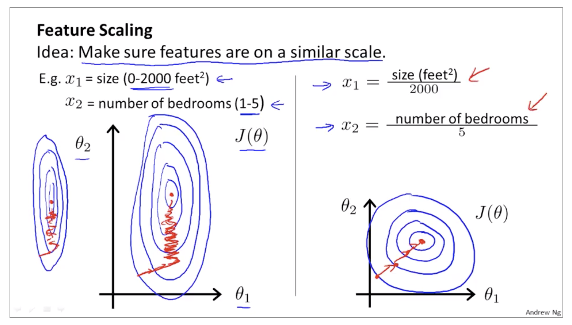
We can speed up gradient descent by having each of our input values in roughly the same range
Feature 끼리 range 차이가 많이나면, contours가 skewed 되기 때문에 converge 하는데 시간이 많이 걸림
Get every feature into approximately a -1 ≤ x_i ≤ 1 range
Feature scaling doesn’t have to be too exact, in order to get GD to run faster
- -0.5 ≤ x_1 ≤ 0.5: O
- -3 ≤ x_2 ≤ 3: O
- -0.0001 ≤ x_3 ≤ 0.0001: X
- -10000 ≤ x_4 ≤ 10000: X
Mean normalization
- Replace x_i with (\(\mu_i\): average value of x, \(s_i\): max value - min value or standard deviation)
  \[x_i := \frac{x_i -\mu_i}{s_i}\]
- Do not apply to \(x_0 = 1\)
  \[x_1 = \frac{size -1000}{2000}, x_2 = \frac{\#bedrooms - 2}{5}\] \[-0.5 \leq x_1 \leq 0.5, -0.5 \leq x_2 \leq 0.5\]

Gradient descent in practice 2 - Learning rate

Gradient descent debugging

\(J(\theta)\) should decrease after every iteration
It turns out to be very difficult to tell how many iterations GD needs to converge
Automatic convergence test
declare convergence if \(J(\theta)\) decreases by less than E(i.g. \(10^{-3}\)) in one iteration
- Andrew Ng은 threshold 값을 설정하는 것도 어려워서 Automatic convergence test는 쓰지 않고 그래프를 그린다고 함
Learning rate(alpha)
- \(J(\theta)\) over shoot 혹은 go up go down: Use smaller alpha
- If alpha is too small: slow convergence
- Andrew Ng은 alpha 값을 특정 값부터 3배씩 증가시켜보면서 \(J(\theta)\) 그래프를 그려본다고 함(i.g. 0.001, 0.003, 0.01, 0.03, 0.1, …)

Features and Polynomial Regression

Defining new features: Housing prices prediction

모델 개선을 위해서 Feature를 조합해서 사용할 수 있음
frontage, depth
- \[h_\theta(x) = \theta_0 + \theta_1 \times frontage + \theta_2 \times depth\]
area = \(frontage \times depth\)
- \[h_\theta(x) = \theta_0 + \theta_1 area\]
Choosing feature is closely related with polynomial regression
- 곡선이 적합한 feature에 polynomial regression 사용(quadratic, cubic, …)
- cubic function
  - \[h_\theta(x) = \theta_0 + \theta_1 area + \theta_2 area^2 + \theta_3 area^3\]
  - Feature scaling: size: 1-1000, size^2: 1-1000,000, size^3: 1-1000,000,000
- sqrt function
  - \[h_\theta(x) = \theta_0 + \theta_1 size + \theta_2 \sqrt{size}\]
  - Feature scaling: size: 1-1000, \(\sqrt{size}\): 1-32

Computing Parameters Analytically

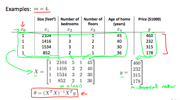
Normal Equation

Method to solve for theta analytically
\(J(\theta) = 0\)의 partial derivative를 theta_0~theta_n 마다 구함(Gradient descent 대신)
one-step learning algorithm

\[\Theta = (X^TX)^{-1}X^Ty\]

Normal Equation vs Gradient descent

장점: Feature scaling 필요 없음, alpha도 선택할 필요 없음, 반복도 없음
단점: \((X^T*X)^{-1}\)을 계산해야 함, \(O(n^3)\): n이 크면 매우 느림
Andrew Ng는 n=10,000부터 GD로 갈아탈지 고민한다고 함, n=1000은 Normal equation 사용
The normal equation method actually do not work for those more sophisticated learning algorithms

Gradient Descent	Normal Equation
Need to choose alpha	No need to choose alpha
Needs many iterations	No need to iterate
\(O (kn^2)\)	\(O(n^3)\) need to calculate inverse of \(X^TX\)
Works well when n is large	Slow if n is very large

Normal Equation Noninvertibility

\[\Theta = (X^TX)^{-1}X^Ty\]

\(X^T \times X\)가 non-invertible(역행렬: X)이면 어떻게 해야 하나?(singular matrix, degenerate matrix)
Octave: pinv(X'*X)*X'*y
- pinv: pseudo-inverse, 역행렬이 없어도 theta 계산 됨
- inv: inverse
X^T*X is non-invertible
- Redundant features(e.g. \(x_1 = size in feet^2\), \(x_2 = size in m^2\))
  - \(X_1 = (3.28)^2*2\), And you can show for those of you that are somewhat advanced in linear Algebra, but if you’re explaining the algebra you can actually show that if your two features are related, are a linear equation like this. Then matrix X transpose X would be non-invertible.
- Too many features(e.g. m ≤ n) train example 수에 비해 feature가 많은 경우
  - Delete some features, or use regularization

Vectorization

for loop를 사용하지 않고 코딩해야 속도가 빠름

← → Top