CS229a - Week 6
Evaluating a Learning Algorithm
Deciding what to try next
Debugging a learning algorithm
if you test your hypothesis on the new set of houses, suppose you find that this is making huge errors in this prediction of the housing prices. The question is what should you then try mixing in order to improve the learning algorithm?
- Get more training examples: But sometimes getting more training data doesn’t actually help
- Try smaller sets of features: To prevent over-fitting (i.g. \(x_1, x_2, ... x_{100}\) select some of them)
- Try getting additional features
- Try adding polynomial features (i.g. \(x_1^2, x_2^2, x_1x_2, etc\))
- Try decreasing or increasing \(\lambda\)
Unfortunately, the most common method that people use to pick one of these is to go by gut feeling. And I have a lot of times, sadly seen people spend, you know, literally 6 months doing one of these avenues that they have sort of at random only to discover six months later that that really wasn’t a promising avenue to pursue.
Machine learning diagnostic
Diagnostics can give guidance as to what might be more fruitful things to try to improve a learning algorithm. Diagnostics can be time-consuming to implement and try, but they can still be a very good use of your time. A diagnostic can sometimes rule out certain courses of action (changes to your learning algorithm) as being unlikely to improve its performance significantly.
Evaluating a hypothesis
So how do you tell if the hypothesis might be overfitting? In simple example we could plot the hypothesis h of x and just see what was going on. But in general for problems with more features than just one feature.
In order to make sure we can evaluate the hypothesis, what we are going to do is split the training data set we have into two portions. The first portion is going to be our usual training set and the second portion is going to be our test set(i.g. training set: 70%, test set: 30%).
- \(m\): number of training set: \((x^{(1)}, y^{(1)}), ...\)
- \(m_{test}\): number of test set: \((x_{test}^{(1)}, y_{test}^{(1)}), ...\)
Suppose an implementation of linear regression (without regularization) is badly overfitting the training set. Then the training error \(J(\Theta)\) to be low and the test error \(J_{test}(\Theta)\) to be high.
That should be better to send a random 70% of your data to the training set and a random 30% of your data to the test set.
Training/testing procedure for linear regression
- Learn parameter \Theta from training data(minimizing training error J(\Theta))
-
Compute test set error:
\[J_{test}(\Theta) = \frac{1}{2m_{test}}\sum_{i=1}^{m_{test}}(h_\Theta(x_{test}^{(i)})-y_{test}^{(i)})^2\]
Training/testing procedure for logistic regression
- Learn parameter \(\Theta\) from training data
- Compute test set error:
-
Misclassification error(0/1 misclassification error):
\[err(h_\theta(x), y) = \begin{cases} 1 & \text{if }h_\theta(x) \ge 0.5, y=0 \text{ or }h_\theta(x) \lt 0.5, y=1 \\ 0 & \text{otherwise} \end{cases}\] \[\text{Test error} = \frac{1}{m_{test}}\sum_{i=1}^{m_{test}}err(h_\Theta(x_{test}^{(i)})-y_{test}^{(i)})\]
Model selection and training/validation/test sets
Suppose you’re left to decide what degree of polynomial to fit a data set. This account model selection process.
Model selection problem
\[h_\theta(x) = \theta_0 + \theta_1x, d=1 \rightarrow J_{test}(\Theta^{(1)}) \\ h_\theta(x) = \theta_0 + \theta_1x + \theta_1x^2, d=2 \rightarrow J_{test}(\Theta^{(2)}) \\ h_\theta(x) = \theta_0 + \theta_1x + ... + \theta_1x^3, d=3 \rightarrow J_{test}(\Theta^{(3)}) \\ ... \\h_\theta(x) = \theta_0 + \theta_1x + ... + \theta_1x^{10}, d=10 \rightarrow J_{test}(\Theta^{(10)})\]- \(d\) = degree of polynomial
In order to select one of these models, I could then see which model has the lowest test set error. And let’s just say for this example that I ended up choosing the fifth order polynomial. Let’s say I want to ask, how well does this model generalize?
But the problem is this will not be a fair estimate of how well my hypothesis generalizes. And the reason is what we’ve done is we’ve fit this extra parameter d, that is this degree of polynomial. And what fits that parameter d, using the test set, namely, we chose the value of d that gave us the best possible performance on the test set. And so, the performance of my parameter vector theta5, on the test set, that’s likely to be an overly optimistic estimate of generalization error.
To address this problem, in a model selection setting, if we want to evaluate a hypothesis, this is what we usually do instead. Given the data set, instead of just splitting into a training test set, what we’re going to do is then split it into three pieces(i.g. training set: 60%, cross validation set: 20%, test set: 20%).
- \(m\): number of training set: \((x^{(1)}, y^{(1)}), ...\)
- \(m_{cv}\): number of cross validation set: \((x_{cv}^{(1)}, y_{cv}^{(1)}), ...\)
- \(m_{test}\): number of test set: \((x_{test}^{(1)}, y_{test}^{(1)}), ...\)
Training error:
\[J_{train}(\Theta) = \frac{1}{2m}\sum_{i=1}^{m}(h_\Theta(x^{(i)})-y^{(i)})^2\]Cross Validation error:
\[J_{cv}(\Theta) = \frac{1}{2m_{cv}}\sum_{i=1}^{m_{cv}}(h_\Theta(x_{cv}^{(i)})-y_{cv}^{(i)})^2\]Test error:
\[J_{test}(\Theta) = \frac{1}{2m_{test}}\sum_{i=1}^{m_{test}}(h_\Theta(x_{test}^{(i)})-y_{test}^{(i)})^2\]And then I’m going to pick the hypothesis with the lowest cross validation error. So for this example, let’s say for the sake of argument, that it was my 4th order polynomial, that had the lowest cross validation error. So in that case I’m going to pick this fourth order polynomial model. so the parameter, is no longer fit to the test set, and so we’ve not saved away the test set, and we can use the test set to measure, or to estimate the generalization error of the model that was selected.
We can now calculate three separate error values for the three different sets using the following method:
- Optimize the parameters in \Theta using the training set for each polynomial degree.
- Find the polynomial degree d with the least error using the cross validation set.
- Estimate the generalization error using the test set with \(J_{test}(\Theta^{(d)})\), (\(d\) = theta from polynomial with lower error);
This way, the degree of the polynomial d has not been trained using the test set.
XXX: K-fold cross-validation이라는 것도 있다. http://karlrosaen.com/ml/learning-log/2016-06-20/
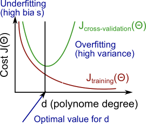
Bias vs Variance
If you run a learning algorithm and it doesn’t do as long as you are hoping, almost all the time, it will be because you have either a high bias problem or a high variance problem, in other words, either an under-fitting problem or an overfitting problem.
Bias/Variance
Training error:
\[J_{train}(\Theta) = \frac{1}{2m}\sum_{i=1}^{m}(h_\Theta(x^{(i)})-y^{(i)})^2\]Cross Validation error:
\[J_{cv}(\Theta) = \frac{1}{2m_{cv}}\sum_{i=1}^{m_{cv}}(h_\Theta(x_{cv}^{(i)})-y_{cv}^{(i)})^2\]Concretely, for the high bias case, that is the case of under-fitting, what we find is that both the cross validation error and the training error are going to be high. In contrast, if your algorithm is suffering from high variance, then if you look here, we’ll notice that J train, that is the training error, is going to be low.
High bias, under-fit
\[J_{train}(\Theta) \text{ will be high} \\ J_{cv}(\Theta) \approx J_{train}(\Theta)\]High variance, over-fit
\[J_{train}(\Theta) \text{ will be low} \\ J_{cv}(\Theta) \gg J_{train}(\Theta)\]Regularization and Bias/Variance
How can we automatically choose a good value for the regularization parameter?
Choosing the regularization parameter \lambda
Model:
\[h_\theta(x) = \theta_0 + \theta_1x + \theta_2x^2 + \theta_3x^3 + \theta_4x^4\]Cost function:
\[J(\Theta) = \frac{1}{2m}\sum_{i=1}^{m}(h_\Theta(x^{(i)})-y^{(i)})^2 + \frac{\lambda}{2m}\sum_{j=1}^n\Theta_j^2\]definitions of J train, J CV and J test are just the average square there one half of the other square record on the training validation of the test set without the extra regularization term.
\[J_{train}(\Theta) = \frac{1}{2m}\sum_{i=1}^{m}(h_\Theta(x^{(i)})-y^{(i)})^2 \\ J_{cv}(\Theta) = \frac{1}{2m_{cv}}\sum_{i=1}^{m_{cv}}(h_\Theta(x_{cv}^{(i)})-y_{cv}^{(i)})^2 \\ J_{test}(\Theta) = \frac{1}{2m_{test}}\sum_{i=1}^{m_{test}}(h_\Theta(x_{test}^{(i)})-y_{test}^{(i)})^2\]So what I usually do is maybe have some range of values of lambda I want to try out. So I might be considering not using regularization or here are a few values I might try lambda considering lambda = 0.01, 0.02, 0.04, and so on. And I usually set these up in multiples of two, until some maybe larger value if I were to do these in multiples of 2 I’d end up with a 10.24. It’s 10 exactly, but this is close enough. So, this gives me maybe 12 different models.
\[\text{Try }\lambda=0 \rightarrow \min_\Theta J(\Theta) \rightarrow \Theta^{(1)} \rightarrow J_{cv}(\Theta^{(1)}) \\ \text{Try }\lambda=0.01 \rightarrow \min_\Theta J(\Theta) \rightarrow \Theta^{(2)} \rightarrow J_{cv}(\Theta^{(2)}) \\ ... \\ \text{Try }\lambda=10 \rightarrow \min_\Theta J(\Theta) \rightarrow \Theta^{(12)} \rightarrow J_{cv}(\Theta^{(12)})\]- Create a list of lambdas.
- Create a set of models with different degrees or any other variants.
- Iterate through the lambdas and for each lambda go through all the models to learn some \(\Theta\).
- Compute the cross validation error using the learned \(\Theta\)(computed with \(\lambda\)) on the \(J_{cv}(\Theta)\) without regularization or \(\lambda = 0\).
- Select the best combo that produces the lowest error on the cross validation set.
- Using the best combo \(\Theta\) and \(\lambda\), apply it on \(J_{test}(\Theta)\) to see if it has a good generalization of the problem.
Learning Curves
Learning curves is a tool that I actually use very often to try to diagnose if a physical learning algorithm may be suffering from bias, sort of variance problem or a bit of both.
Training an algorithm on a very few number of data points (such as 1, 2 or 3) will easily have 0 errors because we can always find a quadratic curve that touches exactly those number of points. Hence:
- As the training set gets larger, the error for a quadratic function increases.
- The error value will plateau out after a certain m, or training set size.
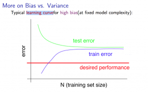
High bias
If a learning algorithm is suffering from high bias, getting more training data will not help much.
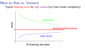
High variance
If a learning algorithm is suffering from high variance, getting more training data is likely to help.
Debugging a learning algorithm
So here is our earlier example of maybe having fit regularized linear regression and finding that it doesn’t work as well as we’re hoping. Is there some way to figure out which of these might be fruitful options?
- Get more training examples: fixes high variance
- Try smaller sets of features: fixes high variance
- Try getting additional features: fixes high bias
- Try adding polynomial features: fixes high bias
- Try decreasing \(\lambda\): fixes high bias
- Try increasing \(\lambda\): fixes high variance
Diagnosing Neural Networks
- A neural network with fewer parameters is prone to under-fitting. It is also computationally cheaper.
- A large neural network with more parameters is prone to overfitting. It is also computationally expensive. In this case you can use regularization (increase \(\lambda\)) to address the overfitting.
Using a single hidden layer is a good starting default. You can train your neural network on a number of hidden layers using your cross validation set. You can then select the one that performs best.
Model Complexity Effects:
- Lower-order polynomials (low model complexity) have high bias and low variance. In this case, the model fits poorly consistently.
- Higher-order polynomials (high model complexity) fit the training data extremely well and the test data extremely poorly. These have low bias on the training data, but very high variance.
- In reality, we would want to choose a model somewhere in between, that can generalize well but also fits the data reasonably well.
If you understood the contents of the last few videos and if you apply them you actually be much more effective already and getting learning algorithms to work on problems and even a large fraction, maybe the majority of practitioners of machine learning here in Silicon Valley today doing these things as their full-time jobs. - Andrew Ng.
XXX: 프로그래밍 과제 풀면서 수식을 코드로 옮기면서 느낀점: Theta(weight), X의 dimension을 생각 안하고 Cost Function이나 Gradient를 계산하면, 간단한 예제에서는 돌아가는 것 같지만 Bias/Variance 균형을 잡기위해서 Model의 Polynomial term의 Degree를 조절할 때 dimension mismatch 같은 문제가 발생한다. 팀 동료로 부터 들은 얘기인데, 수식을 검증하기 위해서 일부러 dimension에 소수(Prime number)를 사용하는게 도움이 된다고 한다. 또 수식에서 Regularization(Lambda term)등을 놓치면 Learning curve상 적당히 학습은 되는 것 같지만, 정확하게 계산되지는 않았다. 프로그래밍 과제에서는 정답이 있으므로 틀렸는지 확인하기 쉬웠지만 실제로는 찾기 어려울 것 같다.
Machine Learning System design
I will actually try to give advice on how to strategize putting together a complex machine learning system.
Building a Spam Classifier
Prioritizing what to work on
I’d like to begin with the issue of prioritizing how to spend your time on what to work on, and I’ll begin with an example on spam classification.
- Supervised learning: Logistic regression
- x: features of email, Choose 100 words indicative of spam or not
- y: spam(1) or not(0)
By the way, even though I’ve described this process as manually picking a hundred words, in practice what’s most commonly done is to look through a training set, and in the training set depict the most frequently occurring n words where n is usually between ten thousand and fifty thousand, and use those as your features.
How to spend your time?
How to spend your time to make it have low error?
- Collect lots of data: https://www.projecthoneypot.org/
- Develop sophisticated features base on email routing information: e.g. fake email headers
- Develop sophisticated features for message body: e.g. discount and discounts be treated as the same word? Features about punctuation?
- Develop sophisticated algorithm to detect misspellings: e.g. m0rtage, med1cine, w4tches
It is difficult to tell which of the options will be most helpful.
- For some learning applications, it is possible to imagine coming up with many different features (e.g. email body features, email routing features, etc.). But it can be hard to guess in advance which features will be the most helpful.
- There are often many possible ideas for how to develop a high accuracy learning system; “gut feeling” is not a recommended way to choose among the alternatives.
Error Analysis
The recommended approach to solving machine learning problems is to
- Start with a simple algorithm, implement it quickly, and test it early on your cross validation data
- Plot learning curves to decide if more data, more features, etc. are likely to help
- Manually examine the errors on examples in the cross validation set and try to spot a trend where most of the errors were made
It is very important to get error results as a single, numerical value. Otherwise it is difficult to assess your algorithm’s performance. For example if we use stemming, which is the process of treating the same word with different forms (fail/failing/failed) as one word (fail), and get a 3% error rate instead of 5%, then we should definitely add it to our model. However, if we try to distinguish between upper case and lower case letters and end up getting a 3.2% error rate instead of 3%, then we should avoid using this new feature. Hence, we should try new things, get a numerical value for our error rate, and based on our result decide whether we want to keep the new feature or not.
Handling Skewed Data
Consider the problem of cancer classification, where we have features of medical patients and we want to decide whether or not they have cancer. So let’s say y equals 1 if the patient has cancer and y equals 0 if they do not. We have trained the progression classifier and let’s say we test our classifier on a test set and find that we get 1 percent error. So, we’re making 99% correct diagnosis. Seems like a really impressive result, right. We’re correct 99% percent of the time.
But now, let’s say we find out that only 0.5 percent of patients in our training test sets actually have cancer. So only half a percent of the patients that come through our screening process have cancer. In this case, the 1% error no longer looks so impressive.
function y = predictCancer(x)
  y = 0; % ignore x, but 99.5% accuracy
end
Precision/Recall(Evaluation metrics)
- true positive: actual: 1, predicted: 1
- true negative: actual: 0, predicted: 0
- false positive: actual: 0, predicted: 1
- false negative: actual: 1, predicted: 0
Precision: Of all patients where we predicted y = 1, what fraction actually has cancer?
\[\frac{\text{true positive}}{\text{true positive} + \text{false positive}}\]Recall: Of all patients that actually have cancer, what fraction did we correctly detect as having cancer?
\[\frac{\text{true positive}}{\text{true positive} + \text{false negative}}\]And by using precision and recall, we find, what happens is that even if we have very skewed classes, it’s not possible for an algorithm to you know, “cheat” and predict y equals 1 all the time, or predict y equals 0 all the time, and get high precision and recall.
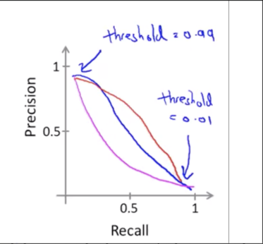
Trading off precision and recall
Logistic regression:
\[0 \le h_\theta(x) \le 1 \\ y = 1 \text{ if } h_\theta(x) \ge 0.5 \\ y=0 \text{ if } h_\theta(x) \lt 0.5\]You’re predicting someone has cancer only when you’re more confident and so you end up with a classifier that has higher precision. Instead of setting the threshold at 0.5, we can set this at 0.7 or 0.9. higher precision, lower recall.
Suppose we want to avoid missing too many actual cases of cancer, so we want to avoid false negatives. Instead of setting the threshold at 0.5, we can set this at 0.3. higher recall, lower precision.
F score
If your goal is to automatically set that threshold to decide what’s really y=1 and y=0, one pretty reasonable way to do that would also be to try a range of different values of thresholds. How to compare precision/recall numbers? Average?
\[Average: \frac{P+R}{2}\]But this turns out not to be such a good solution, because similar to the example we had earlier it turns out that if we have a classifier that predicts y=1 all the time, then if you do that you can get a very high recall, but you end up with a very low value of precision(0.02).
\[F_1Score: 2\frac{PR}{P+R}\] \[P=0 \text{ or } R=0 \rightarrow F_1Score = 0 \\ P=1 \text{ and } R=1 \rightarrow F_1Score = 1\]Using Large Data Sets
Designing a high accuracy learning system
E.g. Classify between confusable words: {to, two, too}, {then, than}
For breakfast I ate _ eggs.
Algorithms
- Perceptron(Logistic regression)
- Winnow
- Memory-based
- Naive Bayes
The performance of the algorithms all pretty much monotonically increase.
Large data rationale
Assume feature \(x \in \R^{n+1}\) has sufficient information to predict y accurately.
- Example: For breakfast I ate _ eggs.
- Counter example: Predict housing price from only size and no other features.
Useful test: Given the input x, can a human expert confidently predict y?
Use a learning algorithm with many parameters(e.g. logistic regression/linear regression with many features; neural network with many hidden units). → Fix high bias problem.
Use a very large training set. → Fix high variance problem.