CS229a - Week 7
Compared to both logistic regression and neural networks, the Support Vector Machine, or SVM sometimes gives a cleaner, and sometimes more powerful way of learning complex non-linear functions.
Large Margin Classification
Optimization Objective
Alternative view of logistic regression
So in logistic regression, we have our familiar form of the hypothesis there and the sigmoid activation function shown on the down.
\[h_\theta(x) = \frac{1}{1+e^{-\theta^Tx}}, z = \theta^Tx\]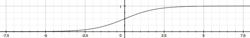
Cost function:
\[-(ylog(h_\theta(x^{(i)}))+(1-y)log(1-h_\theta(x))) \\ = -ylog(\frac{1}{1+e^{-\theta^Tx}})-(1-y)log(1-\frac{1}{1+e^{-\theta^Tx}})\]But turns out, that this will give the support vector machine computational advantages and give us, later on, an easier optimization problem that would be easier for software to solve.
Support vector machine
Logistic regression:
\[\min_\theta \frac{1}{m}[\sum_{i=1}^my^{(i)}(-logh_\theta(x^{(i)})) + (1-y^{(i)})((-log(1-h_\theta(x^{(i)})))]+\frac{\lambda}{2m}\sum_{j=1}^n\theta_j^2\] \[LR: A + \lambda B \\ SVM: CA + B \\ C = \frac{1}{\lambda}\]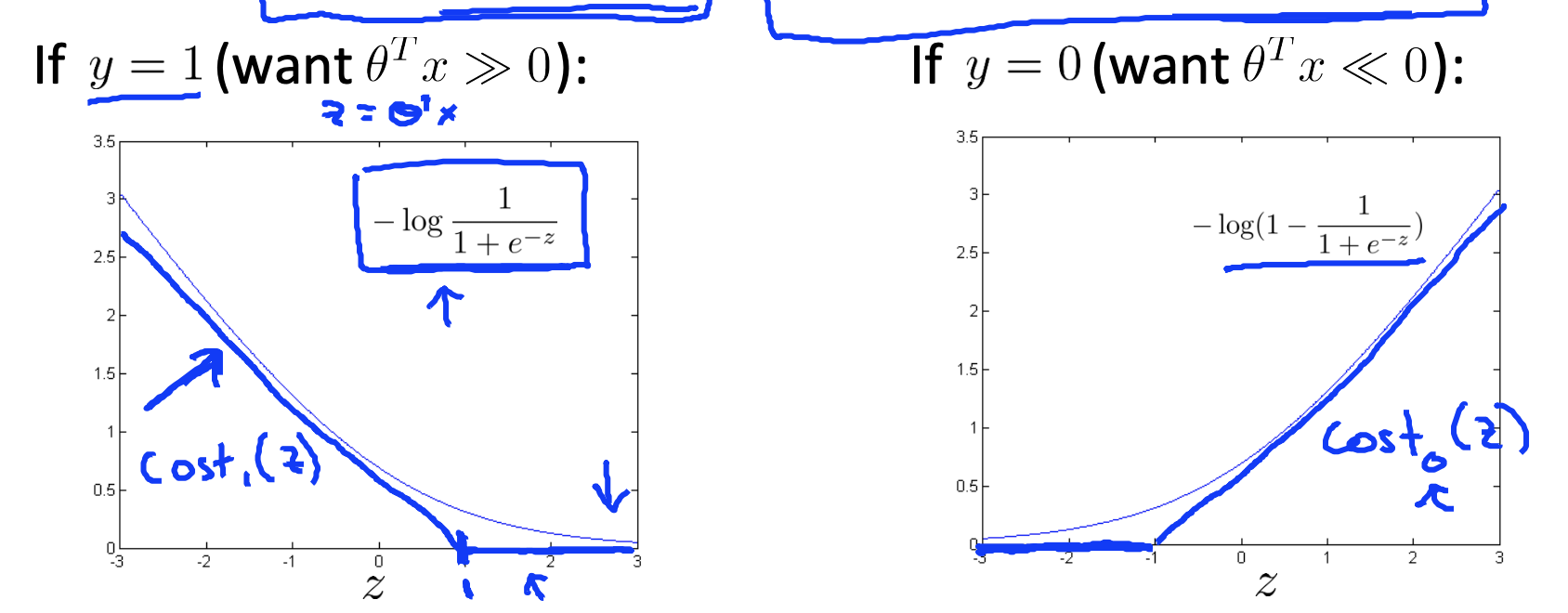
Support vector machine:
\[\min_\theta C\frac{1}{m}[\sum_{i=1}^my^{(i)}cost_1(\theta^Tx^{(i)}) + (1-y^{(i)})(cost_0(\theta^Tx^{(i)}))]+\frac{1}{2}\sum_{j=1}^n\theta_j^2\]SVM Hypothesis:
\[h_\theta(x) \begin{cases} 1 & \text{if }\theta^Tx \ge 0 \\ 0 & \text{otherwise} \end{cases}\]Support vector machines: Large Margin Intuition
Support vector machine:
\[\min_\theta C\frac{1}{m}[\sum_{i=1}^my^{(i)}cost_1(\theta^Tx^{(i)}) + (1-y^{(i)})(cost_0(\theta^Tx^{(i)}))]+\frac{1}{2}\sum_{j=1}^n\theta_j^2\]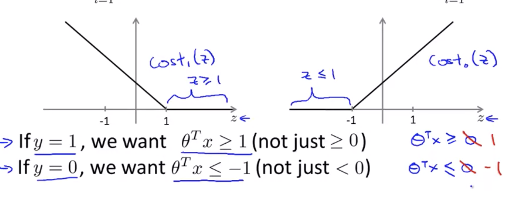
We classify correctly because if theta transpose x is greater than zero our hypothesis will predict zero. And similarly, if you have a negative example, then really all you want is that theta transpose x is less than zero and that will make sure we got the example right.
But the support vector machine wants a bit more than that. It says, you know, don’t just barely get the example right. So then don’t just have it just a little bit bigger than zero. What i really want is for this to be quite a lot bigger than zero say maybe bit greater or equal to one and I want this to be much less than zero. Maybe I want it less than or equal to -1. And so this builds in an extra safety factor or safety margin factor into the support vector machine.
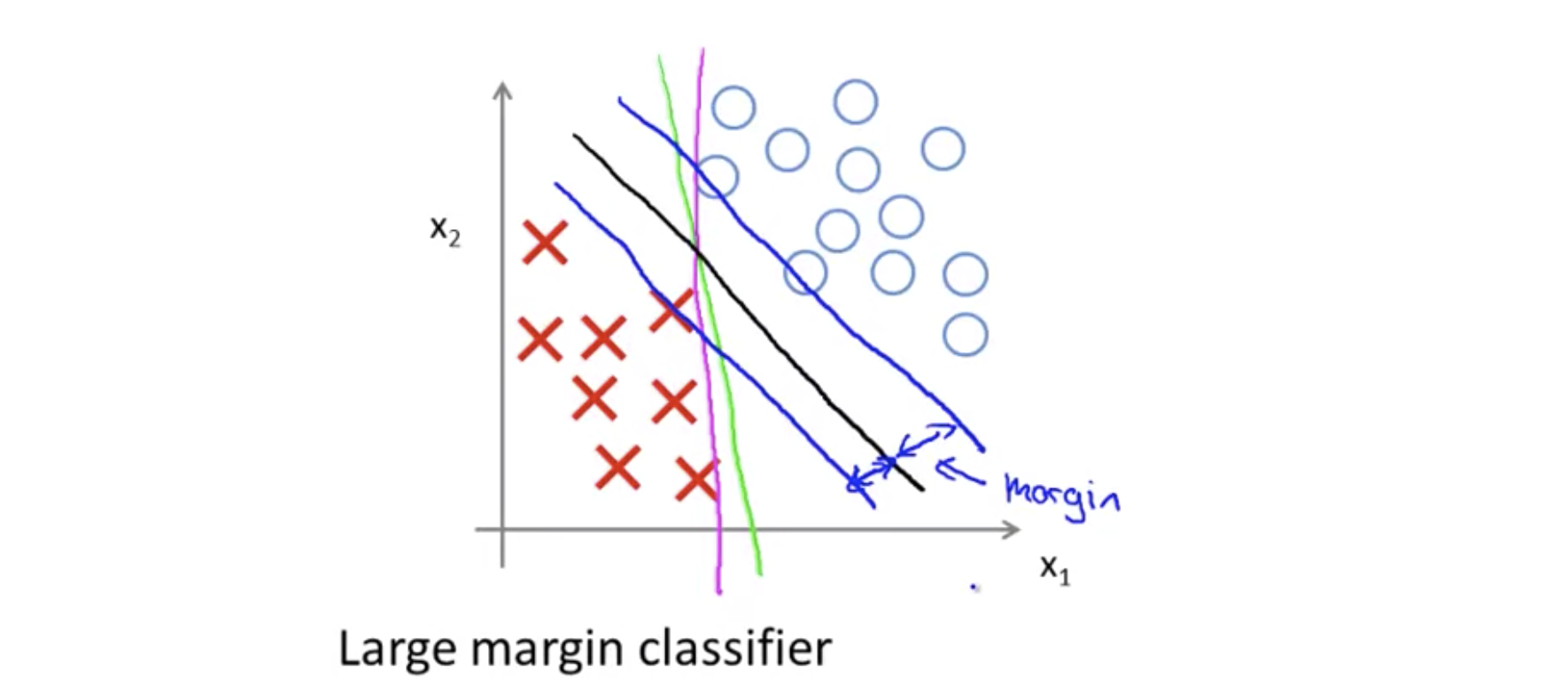
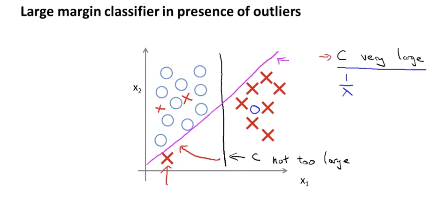
So, if C, if the regularization parameter C were very large, then this is actually what SVM will do, it will change the decision boundary from the black to the magenta one but if C were reasonably small if you were to use the C, not too large then you still end up with this black decision boundary.
Mathematics behind Large margin classification
Vector Inner Product
\[u = \begin{bmatrix} u_1 \\ u_2 \end{bmatrix}, v = \begin{bmatrix} v_1 \\ v_2 \end{bmatrix}\]length of the norm of vector u
\[\left\lVert u \right\rVert = \sqrt{u_1^2 + u_2^2} \in \R\]Inner product:
\[u^Tv = p \cdot \left\lVert u \right\rVert = u_1v_1 + u_2v_2 \\ p = \text{length of projection of } v \text{ onto }u\]If the angle between U and V is less than ninety degrees, then P is the positive length for that red line whereas if the angle of this angle of here is greater than 90 degrees then P here will be negative of the length of the super line of that little line segment right over there.
SVM Decision Boundary
\[\min_\theta\frac{1}{2}\sum_{j=1}^n\theta_j^2 \\ \text{s.t. } \theta^Tx^{(i)} \ge 1 \text{ if } y^{(i)} = 1 \\ \text{ }\theta^Tx^{(i)} \le -1 \text{ if } y^{(i)} = 0\]Simplification: \(\theta_0 = 0\)
\[\min_\theta\frac{1}{2}\sum_{j=1}^n\theta_j^2 = \frac{1}{2}(\theta_1^2 + \theta_2^2) = \frac{1}{2}(\sqrt{\theta_1^2+\theta_2^2})^2 = \frac{1}{2} \left\lVert \theta \right\rVert^2\] \[\theta^Tx^{(i)} = p^{(i)} \cdot \left\lVert \theta \right\rVert = \theta_1x_1^{(i)} + \theta_2x_2^{(i)}\] \[\min_\theta\frac{1}{2}\sum_{j=1}^n\theta_j^2 = \frac{1}{2} \left\lVert \theta \right\rVert^2\\ \text{s.t. } p^{(i)} \cdot \left\lVert \theta \right\rVert \ge 1 \text{ if } y^{(i)} = 1 \\ p^{(i)} \cdot \left\lVert \theta \right\rVert \le -1 \text{ if } y^{(i)} = 0\]where \(p^{(i)}\) is the projection of \(x^{(i)}\) onto the vector \(\theta\). Simplification: \(\theta_0 = 0\)
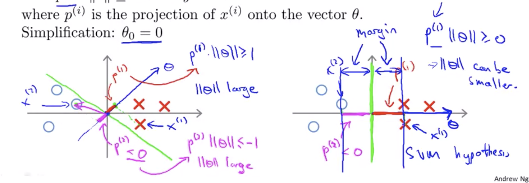
This means is that by choosing the decision boundary shown on the right instead of on the left, the SVM can make the norm of the parameters theta much smaller. So, if we can make the norm of theta smaller and therefore make the squared norm of theta smaller, which is why the SVM would choose this hypothesis on the right instead.
And this is how the SVM gives rise to this large margin certification effect. Mainly, if you look at this green line, if you look at this green hypothesis we want the projections of my positive and negative examples onto theta to be large, and the only way for that to hold true this is if surrounding the green line. There’s this large margin, there’s this large gap that separates
Kernels
I’d like to start adapting support vector machines in order to develop complex nonlinear classifiers. The main technique for doing that is something called kernels.
Terms
- l: landmark, chosen features in training set. i.g. \((x_1^{(i)}, x_2^{(i)})\)
- \(f_1, f_2, f_3\): kernel or similarity function for feature vector
Hypothesis
\[\text{predict 1 when } \theta_0+\theta_1f_1+\theta_2f_2+\theta_3f_3 \ge 0 \\ \text{otherwise } 0\]Kernels and Similarity
Similarity function is, the mathematical term for this, is that this is going to be a kernel function. And the specific kernel I’m using here, this is actually called a Gaussian kernel.
\[f_1 = similarity(x,l^{(1)}) = exp(-\frac{\left\lVert x-l^{(1)} \right\rVert^2}{2\sigma^2}) = exp(-\frac{\sum_{j=1}^n(x_j-l_j^{(1)})^2}{2\sigma^2})\]If \(x \approx l^{(1)}\):
\[f_1 \approx exp(-\frac{0^2}{2\sigma^2}) \approx 1\]If x far from \(l^{(1)}\):
\[f_1 \approx exp(-\frac{(\text{large number})^2}{2\sigma^2}) \approx 0\]Example:
\[l^{(1)} = \begin{bmatrix} 3 \\ 5 \end{bmatrix}, f_1 = exp(-\frac{\left\lVert x-l^{(1)} \right\rVert^2}{2\sigma^2})\]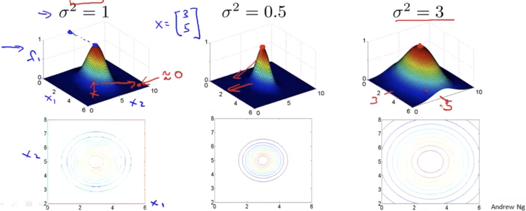
SVM with Kernels
Choosing the landmarks
\[\text{Given } (x^{(1)}, y^{(1)}), (x^{(2)}, y^{(2)}), ...(x^{(m)}, y^{(m)}) \\ \text{Choose } l^{(1)} = x^{(1)}, l^{(2)} = x^{(2)}, ...l^{m}=x^{(m)}\]Feature vectors:
\[f^{(i)} = \begin{bmatrix} f_0^{(i)} \\ f_1^{(i)} \\ f_2^{(i)} \\ ... \\ f_m^{(i)} \end{bmatrix}, f_0^{(i)} = 1\]Hypothesis: Given x
\[\text{compute features } f \in \R^{m+1} \\ \text{Predict } y=1 \text{ if } \Theta^Tf \ge 0\]Training:
\[\min_\theta C\sum_{i=1}^my^{(i)}cost_1(\theta^Tf^{(i)}) + (1-y^{(i)})(cost_0(\theta^Tf^{(i)})) + \frac{1}{2}\sum_{j=1}^n\theta_j^2, n=m\]Vectorized implementation tips:
\[\sum_{j=1}^n\theta_j^2 = \theta^T\theta = \left\lVert \theta \right\rVert^2\]In case your wondering why we don’t apply the kernel’s idea to other algorithms as well like logistic regression, it turns out that if you want, you can actually apply the kernel’s idea and define the source of features using landmarks and so on for logistic regression. But the computational tricks that apply for support vector machines don’t generalize well to other algorithms like logistic regression. And so, using kernels with logistic regression is going too very slow, whereas, because of computational tricks, like that embodied and how it modifies this and the details of how the support vector machine software is implemented, support vector machines and kernels tend go particularly well together.
SVM parameters:
\[C(=\frac{1}{\lambda})\]- Large C: Lower bias, higher variance.
- Small C: Higher bias, lower variance.
- Large \(sigma^2\): Features \(f_i\) vary more smoothly. Higher bias, lower variance.
- Small \(sigma^2\): Features \(f_i\) vary less smoothly. Lower bias, higher variance.
Using an SVM
Just use SVM software package to solve for parameters \theta. But We still need to specify:
- Choice of parameter C
- Choice of kernel(similarity function)
-
No kernel(“linear kernel”): n: large, m: small
\[\text{Predict } y=1 \text{ if, } \theta^Tx \ge 0\] -
Gaussian kernel
\[f_i = exp(-\frac{\left\lVert x-l^{(1)} \right\rVert^2}{2\sigma^2}), \text{where } l^{(l)}=x^{(i)}\]- Need to choose \(\sigma^2\)
- \(n\): small, \(m\): large
-
Depending on what support vector machine software package you use, it may ask you to implement a kernel function, or to implement the similarity function.
And If you have features of very different scales, it is important to perform feature scaling before using the Gaussian kernel.
\[\left\lVert x-l \right\rVert^2 = (x_1-l_1)^2 + (x_2-l_2)^2 + ... + (x_n-l_n)^2\]Other choices of kernel
Note: Not all similarity functions make valid kernels. Similarity function need to satisfy technical condition called Mercer’s Theorem to make sure SVM packages’ optimizations run correctly, and do not diverge.
Many off-the-shelf kernels available:
-
Polynomial kernel: \(k(x,l)\)
\[(X^Tl + constant)^{degree}\] -
More esoteric: String kernel, chi-square kernel, histogram, intersection kernel, …
Multi-class classification
Many SVM packages already have built-in multi-class classification functionality.
Otherwise, use one-vs-all method: Train K SVMs, one to distinguish y = 1 from the rest
Logistic regression vs SVMs
- If n is large relative to m (e.g. n > m, n = 10,000, m = 10 ~ 1000):
- Use logistic regression, or SVM without a kernel(“linear kernel”)
- If n is small, m is intermediate (e.g. n = 1 ~ 1000, m = 10 ~ 10,000):
- Use SVM with Gaussian kernel
- If n is small, m is large (e.g. n = 1 ~ 1000, m = 50,000 ~):
- Create/add more features, then use logistic regression or SVM without a kernel
the guidelines are a bit vague, I’m still not entirely sure, should I use this algorithm or that algorithm, that’s actually okay. When I face a machine learning problem, you know, sometimes its actually just not clear whether that’s the best algorithm to use, but as you saw in the earlier videos, really, you know, the algorithm does matter, but what often matters even more is things like, how much data do you have. And how skilled are you, how good are you at doing error analysis and debugging learning algorithms, figuring out how to design new features and figuring out what other features to give you learning algorithms and so on. And often those things will matter more than what you are using logistic regression or an SVM. But having said that, the SVM is still widely perceived as one of the most powerful learning algorithms, and there is this regime of when there’s a very effective way to learn complex non linear functions. And so I actually, together with logistic regressions, neural networks, SVM’s, using those to speed learning algorithms you’re I think very well positioned to build state of the art you know, machine learning systems for a wide region for applications and this is another very powerful tool to have in your arsenal. One that is used all over the place in Silicon Valley, or in industry and in the Academia, to build many high performance machine learning system. - Andrew Ng.