CS229a - Week 10
Gradient Descent with Large Datasets
Learning with Large Datasets
One of the reasons that learning algorithms work so much better now than even say, 5-years ago, is just the amount of data that we have now and that we can train our algorithms on. So why do we want to use such large data sets? We’ve already seen that one of the best ways to get a high performance machine learning system, is if you take a low-bias learning algorithm, and train that on a lot of data.
But learning with large data sets comes with its own unique problems, specifically, computational problems. Let’s say your training set size is M equals 100,000,000.
\[\theta_j := \theta_j - \alpha \sum_{i=1}^m (h_\theta(x^{(i)})-y^{(i)}) x_j^{(i)}\]You need to carry out a summation over a hundred million terms, in order to compute these derivatives terms and to perform a single step of decent.
Of course, before we put in the effort into training a model with a hundred million examples, We should also ask ourselves, well, why not use just a thousand examples. Suppose you are facing a supervised learning problem and have a very large dataset (m = 100,000,000).
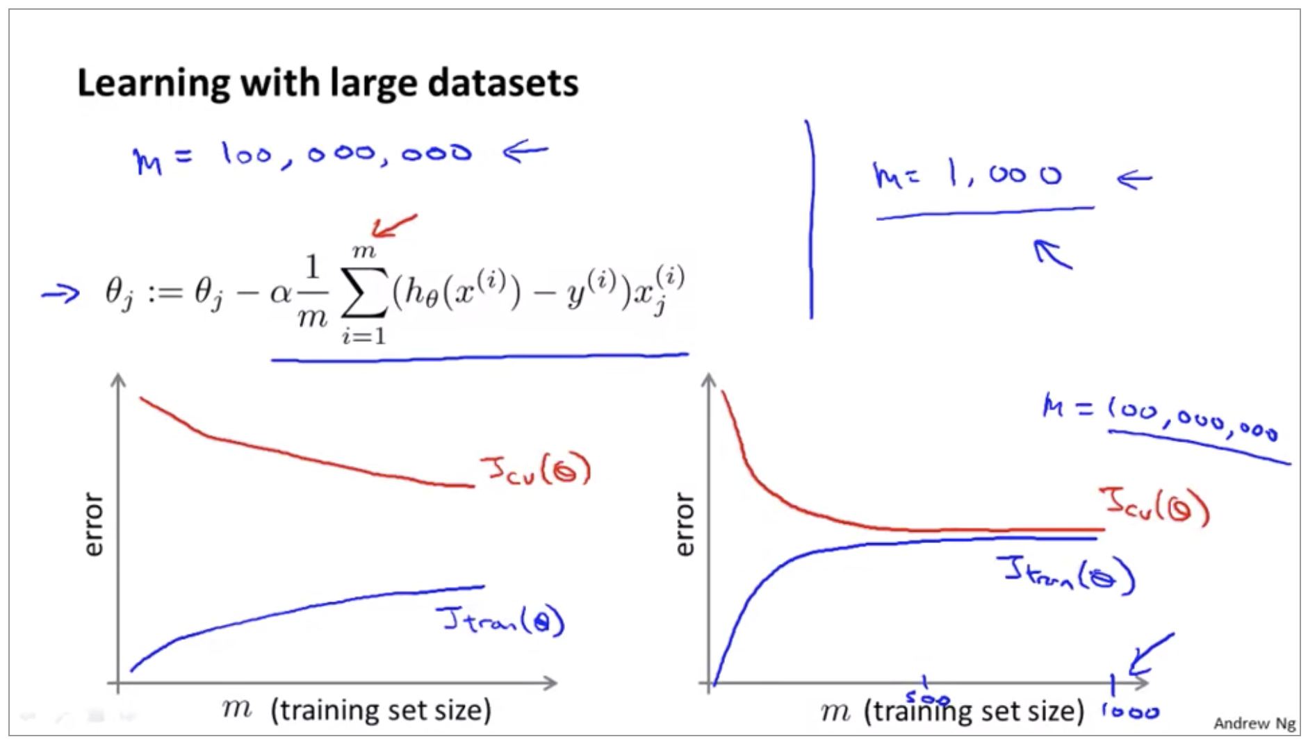
How can you tell if using all of the data is likely to perform much better than using a small subset of the data (say m = 1,000)? Plot a learning curve for a range of values of m and verify that the algorithm has high variance when m is small.
Stochastic gradient descent
When we have a very large training set, gradient descent becomes a computationally very expensive procedure.
Batch gradient descent
Hypothesis:
\[h_\theta = \sum_{j=0}^n \theta_jx_j\]Cost function:
\[J_{train}(\Theta) = \frac{1}{2m}\sum_{i=1}^{m}(h_\Theta(x^{(i)})-y^{(i)})^2\]Gradient descent Repeat(for every j = 0, …, n):
\[\theta_j := \theta_j - \alpha \sum_{i=1}^m (h_\theta(x^{(i)})-y^{(i)}) x_j^{(i)}\]If we have hundred million examples ,then computing this derivative term can be very expensive, because the surprise, summing over all m examples. To give the algorithm a name, this particular version of gradient descent is also called Batch gradient descent.
Stochastic gradient descent
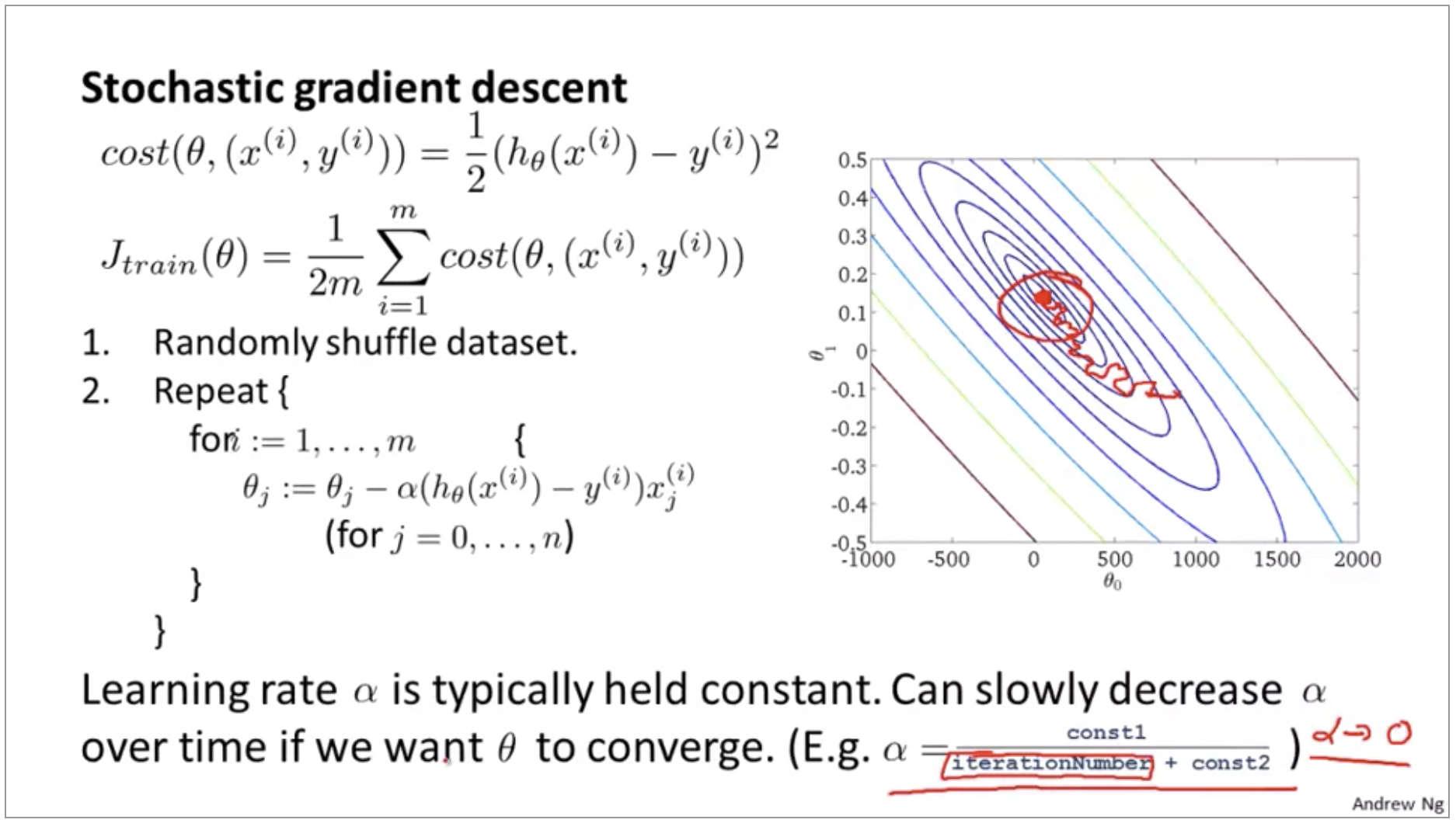
Cost function:
\[cost(\theta,(x^{(i)}, y^{(i)})) = \frac{1}{2}(h_\Theta(x^{(i)})-y^{(i)})^2 \\ J_{train}(\Theta) = \frac{1}{2m}\sum_{i=1}^{m}cost(\theta,(x^{(i)}, y^{(i)}))\]Gradient descent:
- Randomly shuffle training examples
-
Repeat {
for i := 1, …, m {
\[\theta_j := \theta_j - \alpha (h_\theta(x^{(i)})-y^{(i)}) x_j^{(i)} \\ (\text{for } j = 0, ..., n)\]}
}
Stochastic gradient descent is a lot like descent but rather than wait to sum up these gradient terms over all m training examples, what we’re doing is we’re taking this gradient term using just one single training example and we’re starting to make progress in improving the parameters already.
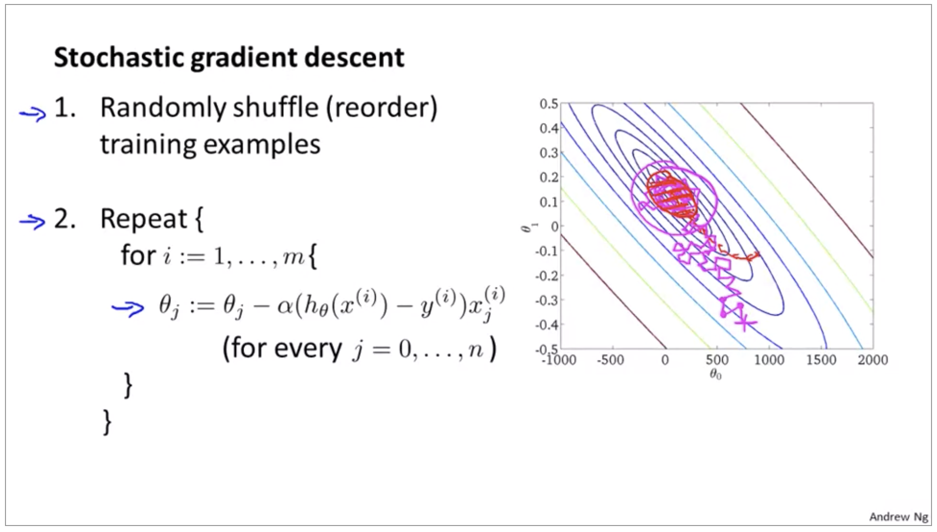
As you run Stochastic gradient descent, what you find is that it will generally move the parameters in the direction of the global minimum, but not always. And so take some more random-looking, circuitous path to watch the global minimum. And in fact as you run Stochastic gradient descent it doesn’t actually converge in the same same sense as Batch gradient descent does and what it ends up doing is wandering around continuously in some region that’s in some region close to the global minimum, but it doesn’t just get to the global minimum and stay there. But in practice this isn’t a problem because, you know, so long as the parameters end up in some region there maybe it is pretty close to the global minimum.
Mini-batch gradient descent
- Batch gradient descent: Use all m examples in each iteration
- Stochastic gradient descent: Use 1 example in each iteration
- Mini-batch gradient descent: Use b examples in each iteration(typical range: 2~100)
So we have again data with 300 million training examples, then what we’re saying is after looking at just the first 10 examples we can start to make progress in improving the parameters theta so we don’t need to scan through the entire training set. We just need to look at the first 10 examples and this will start letting us make progress and then we can look at the second ten examples and modify the parameters a little bit again and so on. So, that is why Mini-batch gradient descent can be faster than batch gradient descent.
So, why do we want to look at b examples at a time rather than look at just a single example at a time as the Stochastic gradient descent? The answer is in vectorization. In particular, Mini-batch gradient descent is likely to outperform Stochastic gradient descent only if you have a good vectorized implementation.
Stochastic Gradient Descent Convergence
Back when we were using batch gradient descent, our standard way for making sure that gradient descent was converging was we would plot the optimization cost function as a function of the number of iterations. So that was the cost function and we would make sure that this cost function is decreasing on every iteration.
Batch gradient descent:
-
Plot \(J_{train}(\theta)\) as function of the number of iterations of gradient decent
\[J_{train}(\theta) = \frac{1}{2m}\sum_{i=1}^m(h_\theta(x^{(i)})-y^{(i)})^2\]
Stochastic gradient descent:
\[cost(\theta,(x^{(i)},y^{(i)})) = \frac{1}{2}(h_\theta(x^{(i)})-y^{(i)})^2\]- During learning, compute \(cost(\theta, (x^{(i)}, y^{(i)}))\) before updating \(\theta\) using \((x^{(i)}, y^{(i)})\).
- Every 1000 iterations (say), plot \(cost(\theta, (x^{(i)}, y^{(i)}))\) averaged over the last 1000 examples processed by algorithm
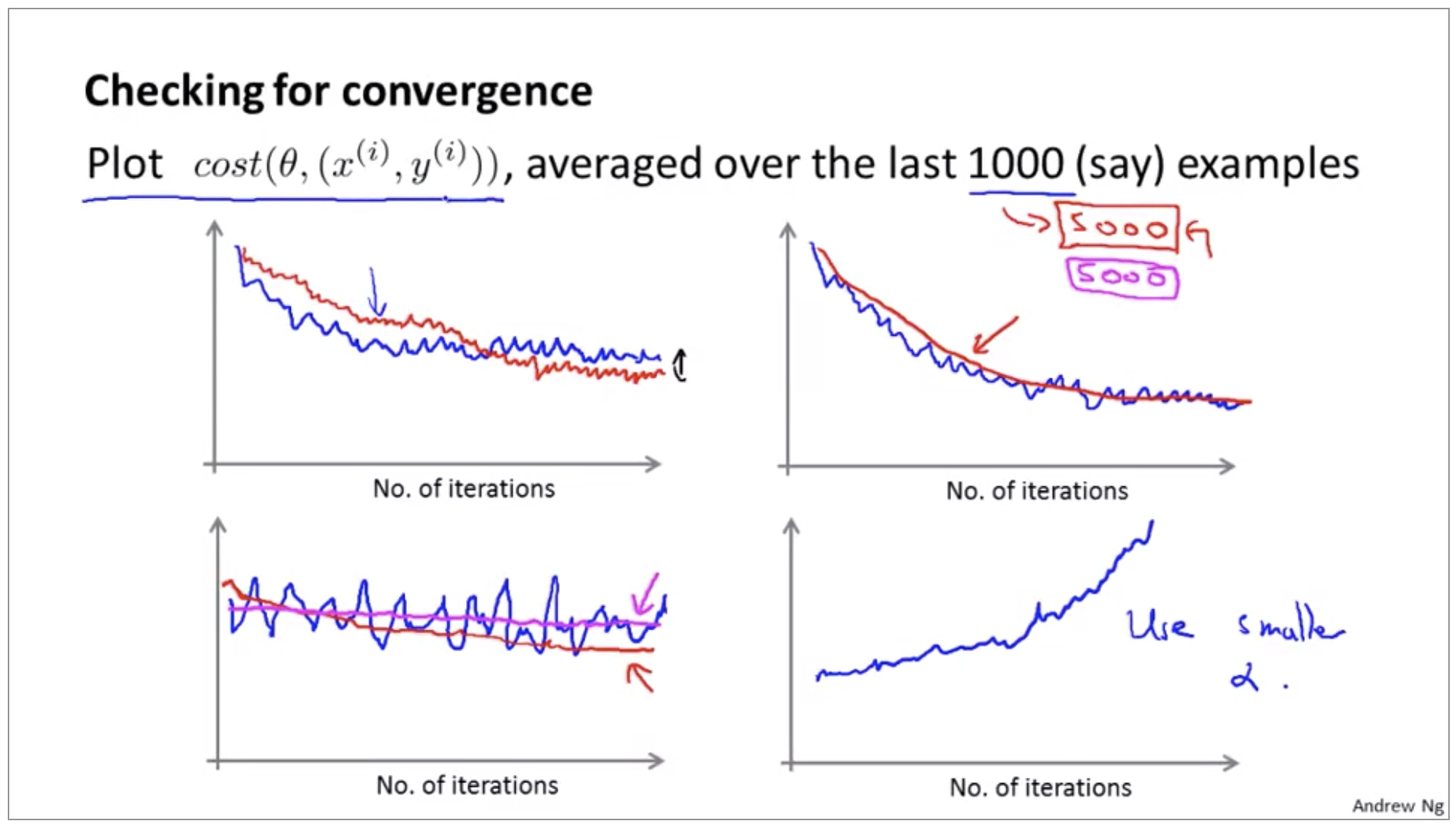
Typically this process of decreasing alpha slowly is usually not done and keeping the learning rate alpha constant is the more common application of stochastic gradient descent although you will see people use either version.
Advanced Topic
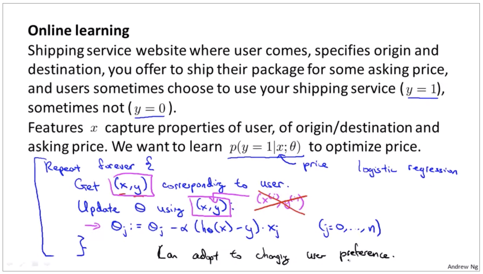
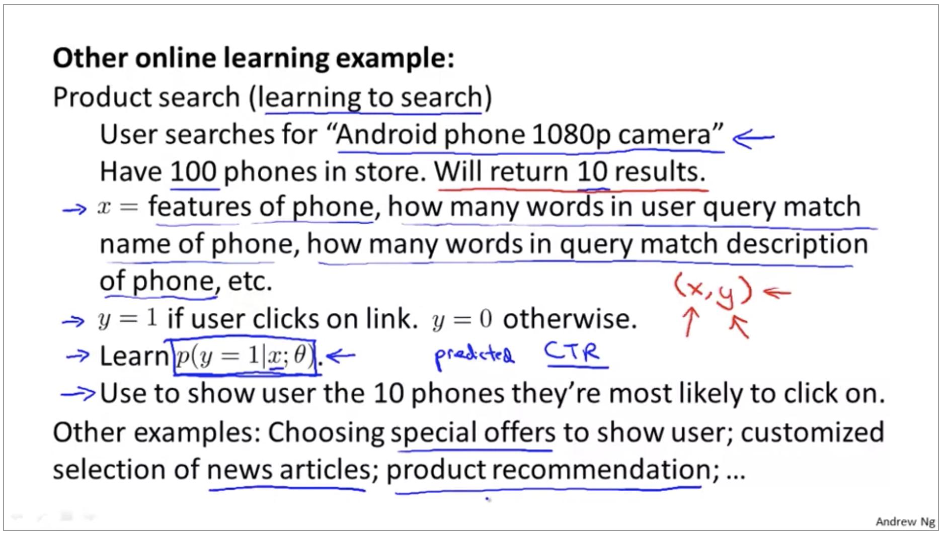
Online Learning
The online learning setting allows us to model problems where we have a continuous flood or a continuous stream of data coming in and we would like an algorithm to learn from that.
Map Reduce and Data Parallelism
Map-reduce
Batch gradient descent:
\[\theta_j := \theta_j - \alpha \frac{1}{400} \sum_{i=1}^{400}(h_\theta(x^{(i)})-y^{(i)})x_j^{(i)}\]-
Machine 1:
\[(x^{(1)}, y^{(1)}), ..., (x^{(100)}, y^{(100)}) \\ temp_j^{(1)} = \sum_{i=1}^{100} (h_\theta(x^{(i)})-y^{(i)})x_j^{(i)}\] -
Machine 2:
\[(x^{(101)}, y^{(101)}), ..., (x^{(200)}, y^{(200)}) \\ temp_j^{(2)} = \sum_{i=101}^{200} (h_\theta(x^{(i)})-y^{(i)})x_j^{(i)}\] -
Machine 3:
- Machine 4:
Combine temp:
\[\theta_j := \theta_j - \alpha \frac{1}{400}(temp_j^{(1)} + temp_j^{(2)} + temp_j^{(3)} + temp_j^{(4)})\]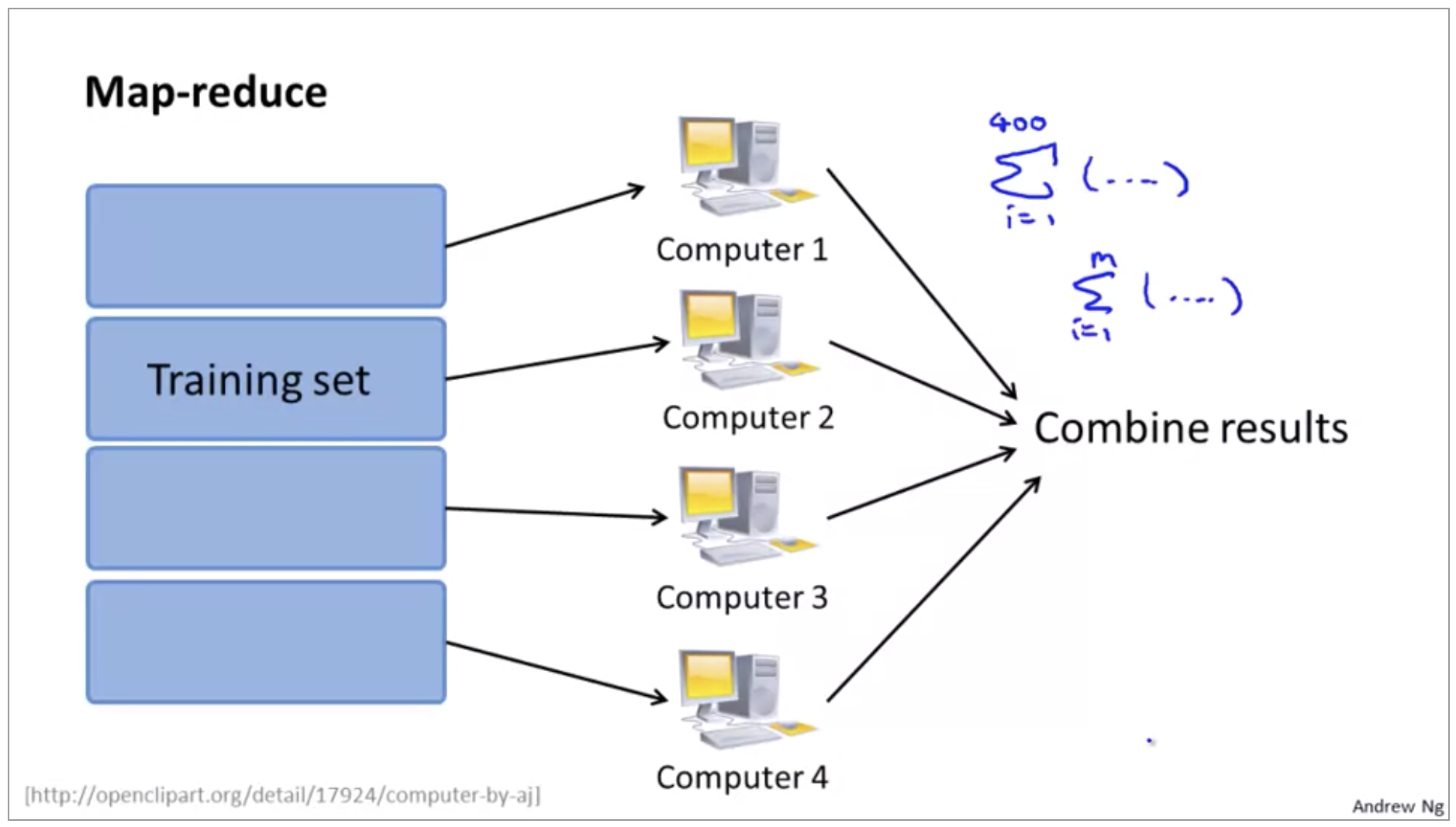
Map-reduce and summation over the training set
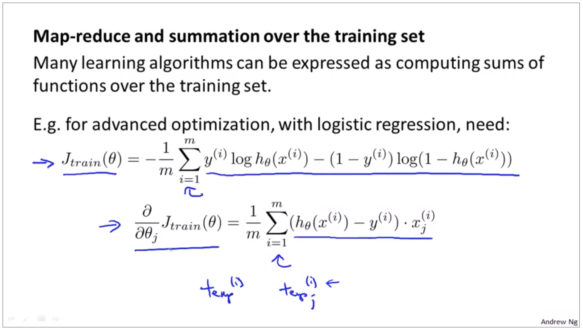
Compute forward propagation and back propagation on 1/n of the data to compute the derivative with respect to that 1/n of the data.
More broadly, by taking other learning algorithms and expressing them in sort of summation form or by expressing them in terms of computing sums of functions over the training set, you can use the MapReduce technique to parallelize other learning algorithms as well, and scale them to very large training sets.
Sometimes you can just implement you standard learning algorithm in a vectorized fashion and not worry about parallelization and numerical linear algebra libraries could take care of some of it for you.