CS229a - Week 9
Density Estimation
Problem Motivation
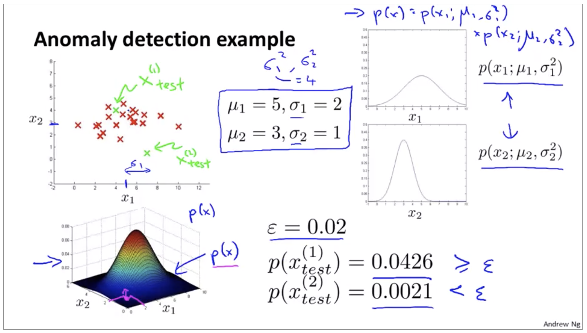
Aircraft engine features:
- \(x_1\) = heat generated
- \(x_2\) = vibration intensity
-
Dataset:
\[\{x^{(1)}, x^{(2)}, ..., x^{(m)}\}\] - New engine: \(x_{test}\)
Fraud detection:
- \(x^{(i)}\): features of user i’s activities
- Model \(p(x)\) from data.
-
Identify unusual users by checking which have:
\[p(x) \le \epsilon\]
Monitoring computers in a data center:
- \(x^{(i)}\) = features of machine i
- \(x_1\) = memory use
- \(x_2\) = number of disk accesses/sec
- \(x_3\) = CPU load
- \(x_4\) = CPU load/network traffic
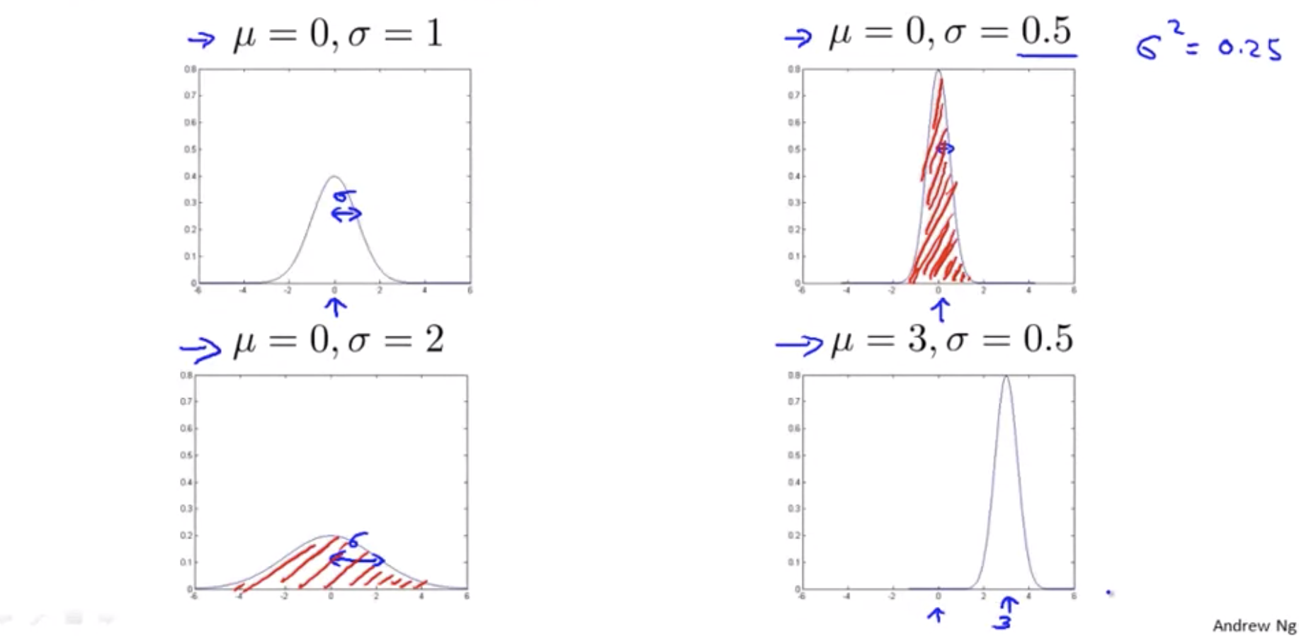
Gaussian Distribution(Normal Distribution)
If x is a distributed Gaussian with mean \mu, variance: \sigma^2.
\[x \sim N(\mu,\sigma^2)\]- \(\mu\): mean
- \(\sigma\): standard deviation
- \(\sigma^2\): variance
Some of you may have seen the formula here where this is M-1 instead of M so this first term becomes 1/M-1 instead of 1/M. In machine learning people tend to learn 1/M formula but in practice whether it is 1/M or 1/M-1 it makes essentially no difference assuming M is reasonably large.
Algorithm
Training set:
\[\{x^{(1)}, x^{(2)}, ..., x^{(m)}\}, x \in \R^n\]The problem of density estimation:
\[p(x) = p(x_1;\mu_1,\sigma_1^2)p(x_2;\mu_2,\sigma_2^2)...p(x_n;\mu_n,\sigma_n^2) \\ = \Pi_{j=1}^n p(x_j;\mu_j,\sigma_j^2)\]- Capital Greek alphabet pi is product symbol
- p of x is probability of x, sometimes called the problem of density estimation
Anomaly detection algorithm
- Choose features \(x_i\) that you think might be indicative of anomalous examples
-
Fit parameters: \(\mu_1,...,\mu_n,\sigma_1^2,...,\sigma_n^2\)
\[\mu_j = \frac{1}{m} \sum_{i=1}^m x^{(i)}_j \\ \sigma^2_j = \frac{1}{m} \sum_{i=1}^m (x^{(i)}_j - \mu_j)^2\] -
Given new example x, compute p(x):
\[p(x) = \Pi_{j=1}^n p(x_j;\mu_j,\sigma_j^2) \\ = \Pi_{j=1}^n\frac{1}{\sqrt{2\pi}\sigma_j}exp(-\frac{(x_j-\mu_j)^2}{2\sigma_j^2})\] \[\text{Anomaly if } p(x) \lt \epsilon\]
Developing and Evaluating an Anomaly Detection System
You need to often make a lot of choices like, you know, choosing what features to use and then so on. And making decisions about all of these choices is often much easier, and if you have a way to evaluate your learning algorithm that just gives you back a number.
Aircraft engines motivating example
We have manufactured 10,000 examples of engines that, as far as we know we’re perfectly normal and let’s say that we end up getting features, getting 24 to 28 anomalous engines as well.
- 10000: good(normal) engines
- 20: flawed engines(anomalous)
A fairly typical way to split it into the training set, cross validation set and test set would be as follows.
- Training set: 6000 good engines
- Cross validation set: 2000 good engines(\(y=0\)), 10 anomalous(\(y=1\))
- Test set: 2000 good engines(\(y=0\)), 10 anomalous(\(y=1\))
Algorithm evaluation
- Fit model \(p(x)\) on training set
-
On a cross validation/test example x, predict:
\[y = \begin{cases} 1 & \text{if } p(x) \lt \epsilon \text{ (anomaly)} \\ 0 & \text{if } p(x) \ge \epsilon \text{ (normal)} \end{cases}\] - Possible evaluation metrics:
- True positive, false positive, false negative, true negative
- Precision/Recall
- \(F_1\) - score Is classification accuracy a good way to measure the algorithm’s performance? No, because of skewed classes (so an algorithm that always predicts y = 0 will have high accuracy).because of skewed classes (so an algorithm that always predicts y = 0 will have high accuracy). Can also use cross validation set to choose parameter \(\epsilon\)
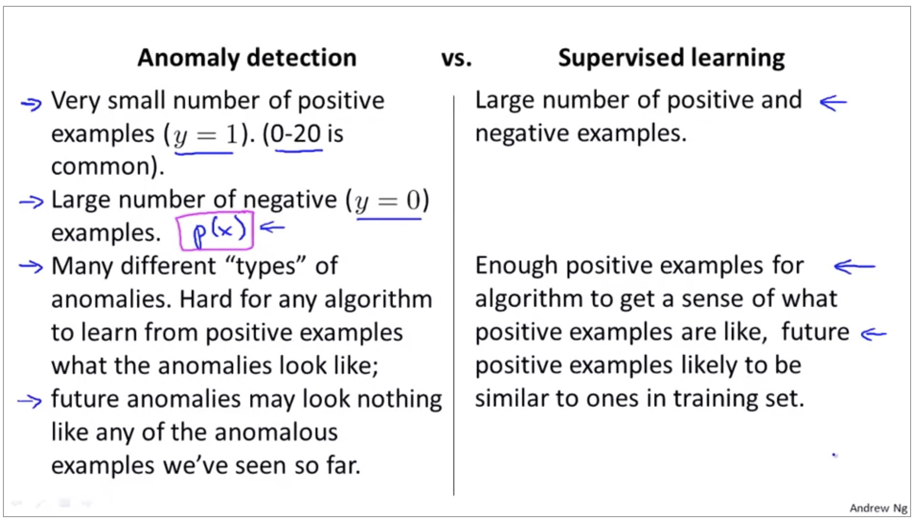
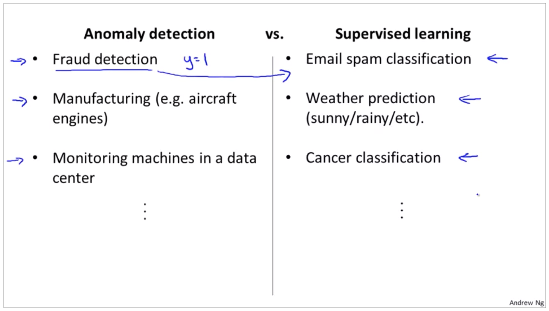
Anomaly Detection vs Supervised Learning
And so, the question then arises of, and if we have the label data, that we have some examples and know the anomalies, and some of them will not be anomalies. Why don’t we just use a supervisor on half of them? So why don’t we just use logistic regression, or a neural network to try to learn directly from our labeled data to predict whether Y equals one or Y equals 0.
Choosing what features to use
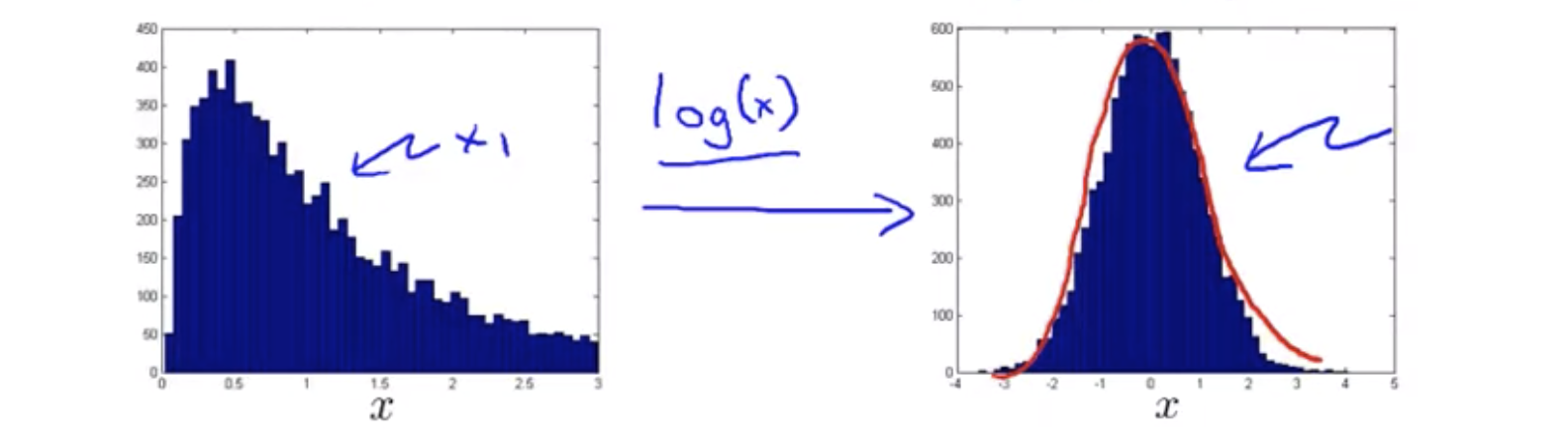
If you plot a histogram with the data, and find that it looks pretty non-Gaussian, it’s worth playing around a little bit with different transformations like these(\(log(x), x^\frac{1}{2}, ...\)), to see if you can make your data look a little bit more Gaussian, before you feed it to your learning algorithm, although even if you don’t, it might work okay. But I usually do take this step.
Error analysis for anomaly detection
This is really similar to the error analysis procedure that we have for supervised learning, where we would train a complete algorithm, and run the algorithm on a cross validation set, and look at the examples it gets wrong, and see if we can come up with extra features to help the algorithm do better on the examples that it got wrong in the cross-validation set.
Try coming up with more features to distinguish between the normal and the anomalous examples.
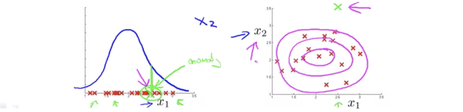
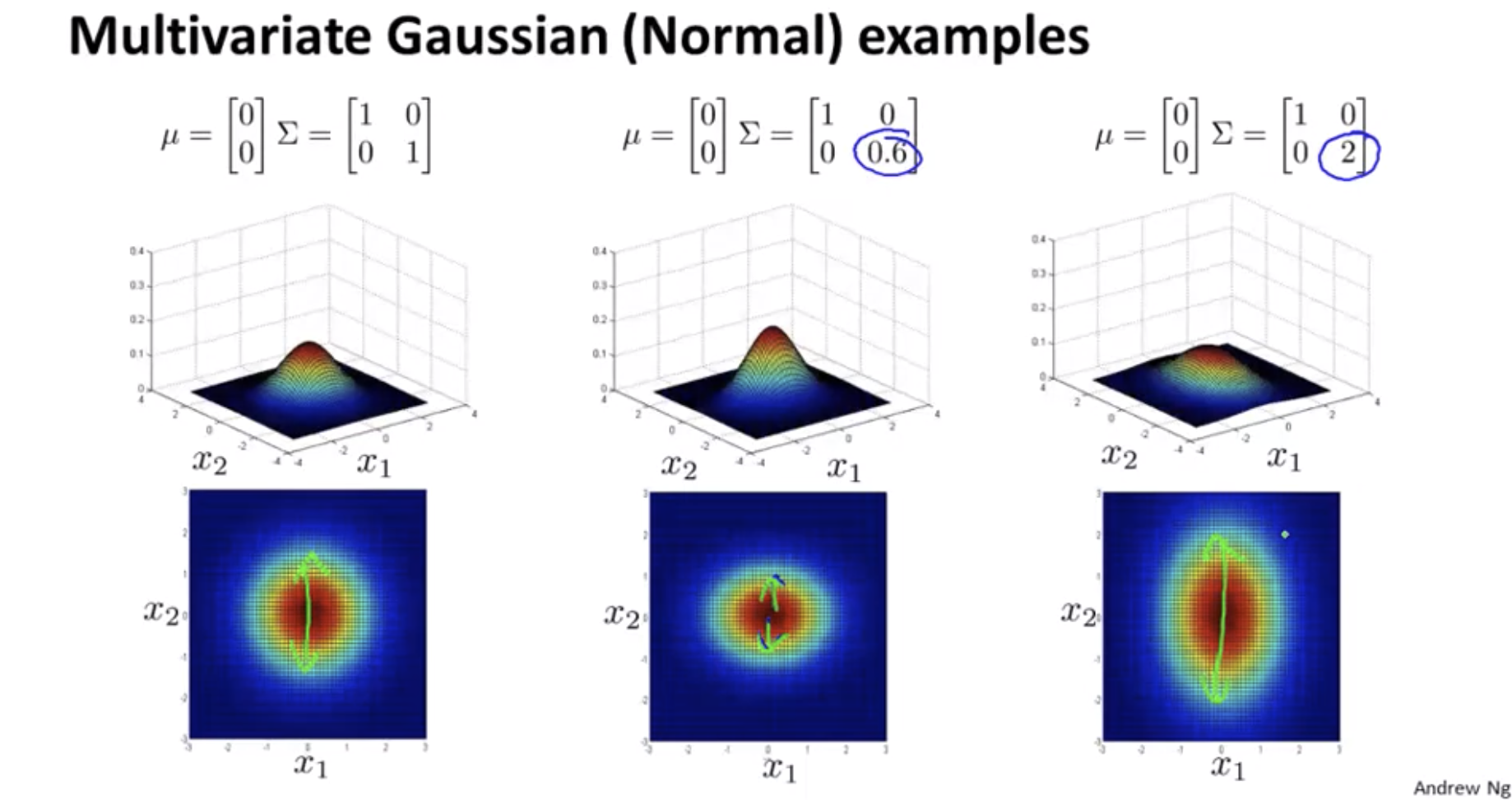
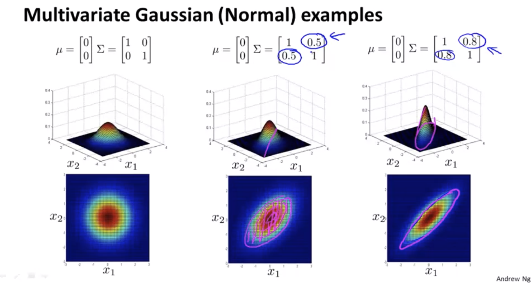
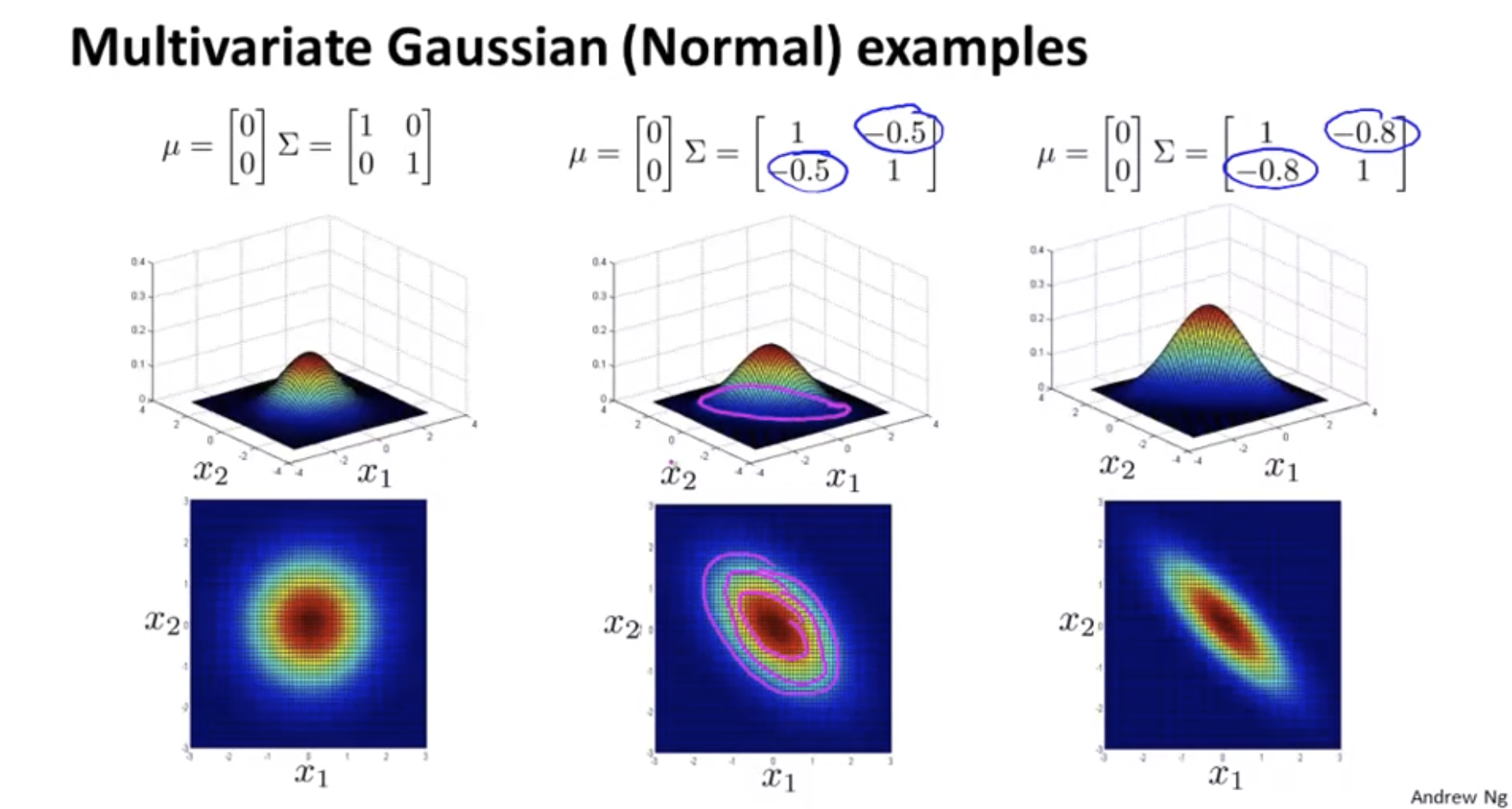
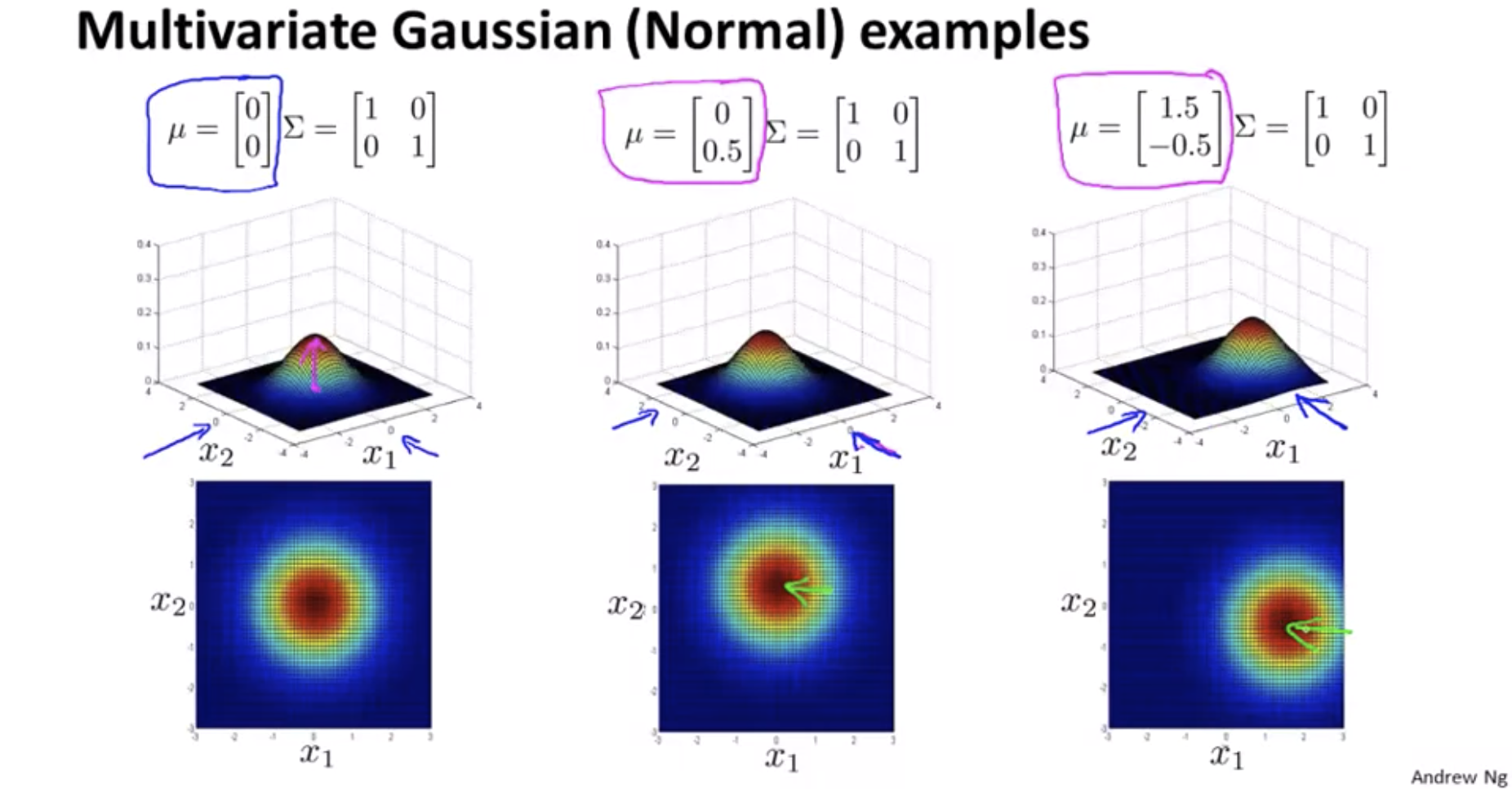
Multivariate Gaussian Distribution
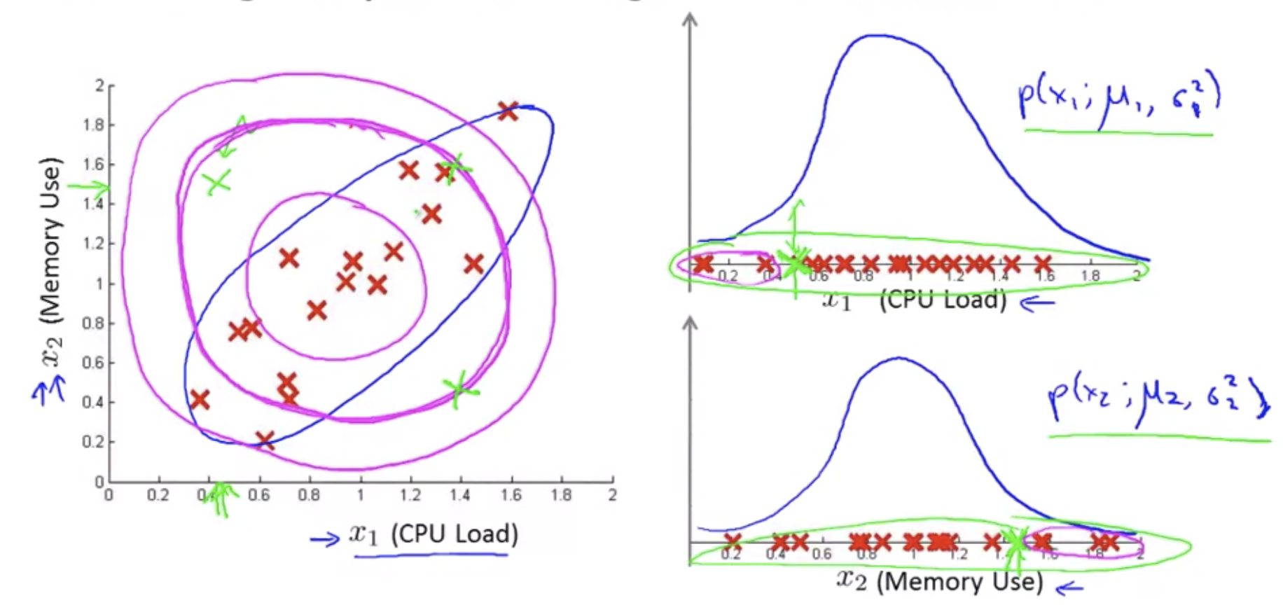
In order to fix this, we can, we’re going to develop a modified version of the anomaly detection algorithm, using something called the multivariate Gaussian distribution also called the multivariate normal distribution.
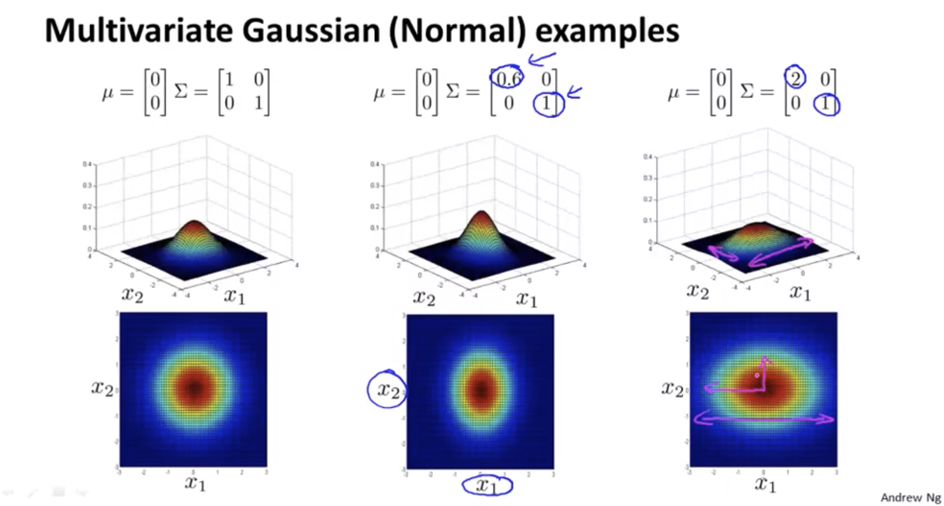
Multivariate Gaussian distribution
\[p(x;\mu,\Sigma) = \frac{1}{(2\pi)^{\frac{n}{2}}|\Sigma|^{\frac{1}{2}}}exp(-\frac{1}{2}(x-\mu)^T\Sigma^{-1}(x-\mu))\] \[|\Sigma|: \text{ determinant of } \Sigma\]https://en.wikipedia.org/wiki/Determinant
How do I try to estimate my parameters mu and sigma?
\[\mu = \frac{1}{m}\sum_{i=1}^m x^{(i)}, \Sigma = \frac{1}{m}\sum_{i=1}^m (x^{(i)}-\mu)(x^{(i)}-\mu)^T\]Original model vs Multivariate Gaussian
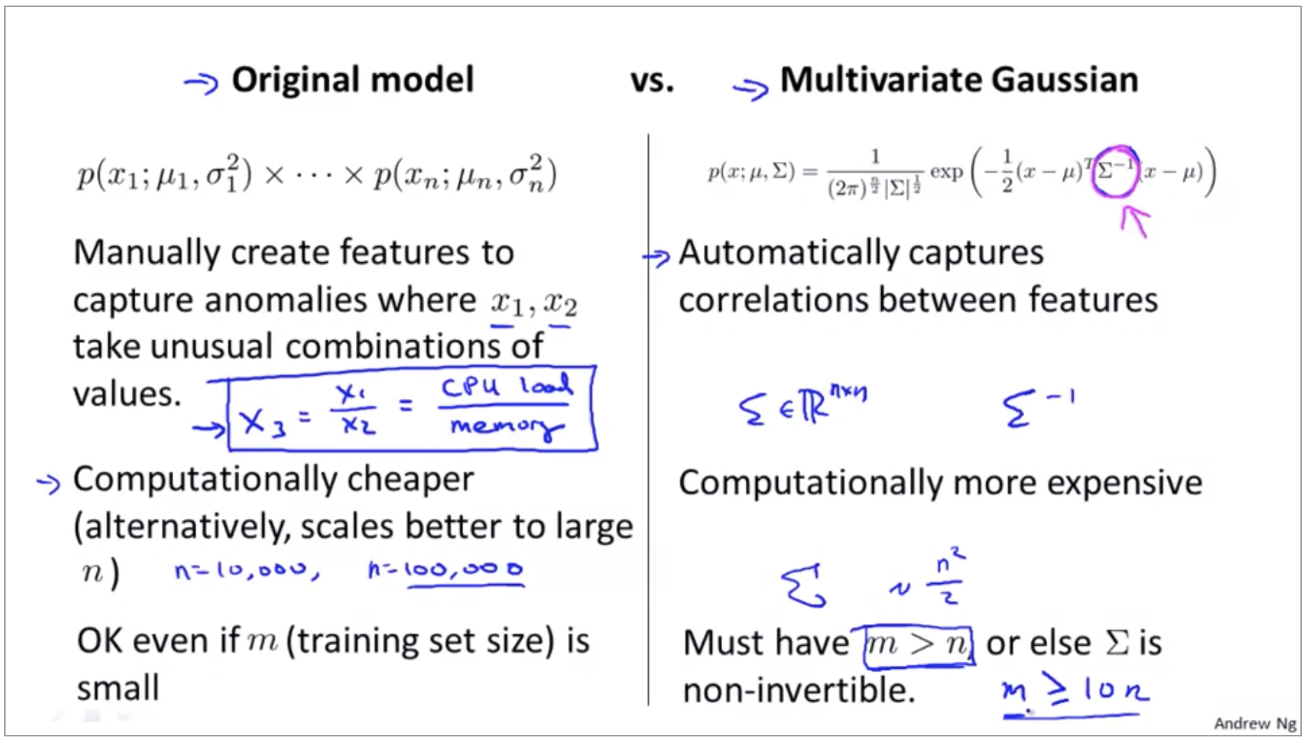
The original model corresponds to a multivariate Gaussian where the contours of \(p(x)\) are axis-aligned.
Recommender Systems
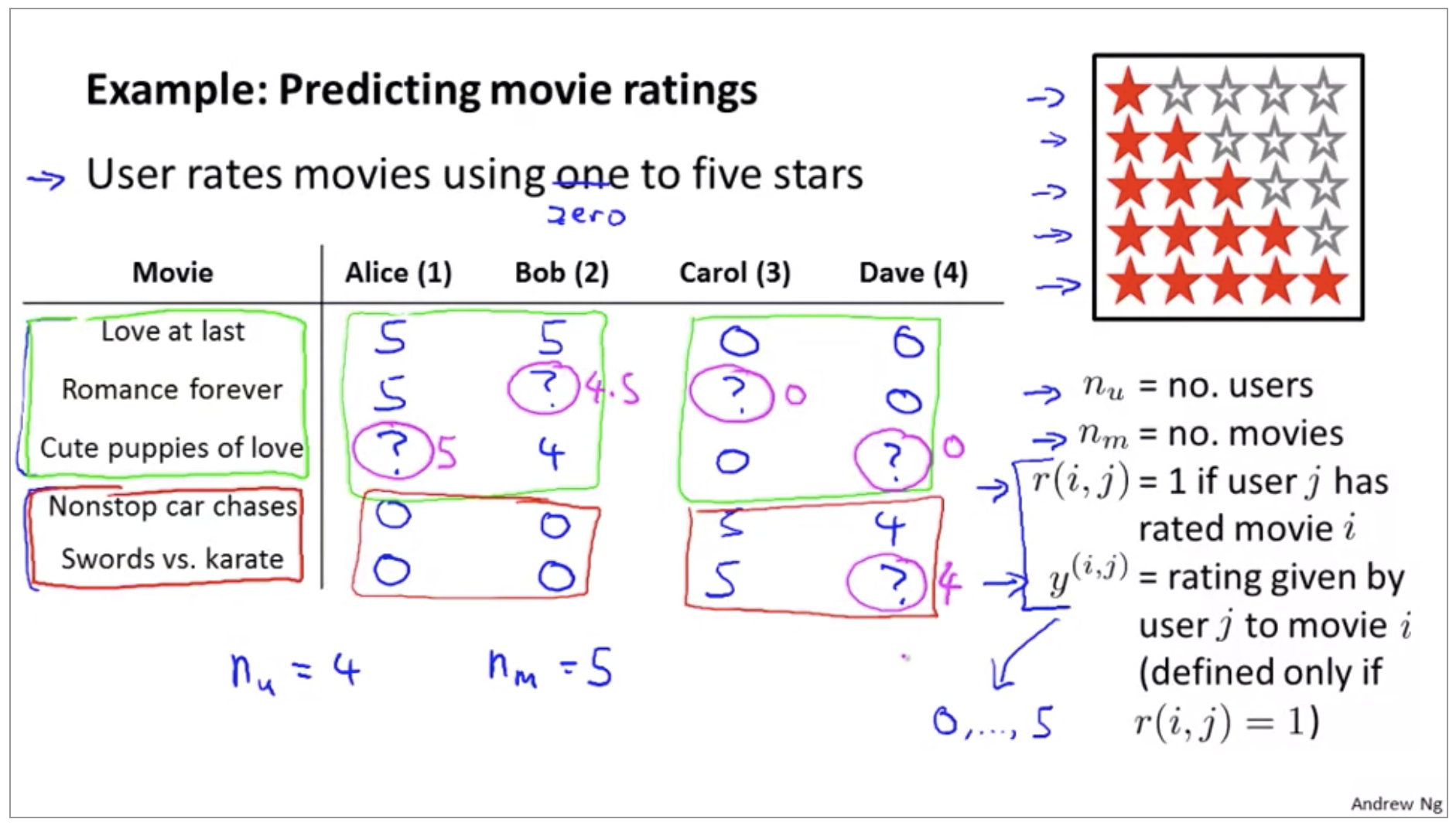
Predicting Movie Ratings
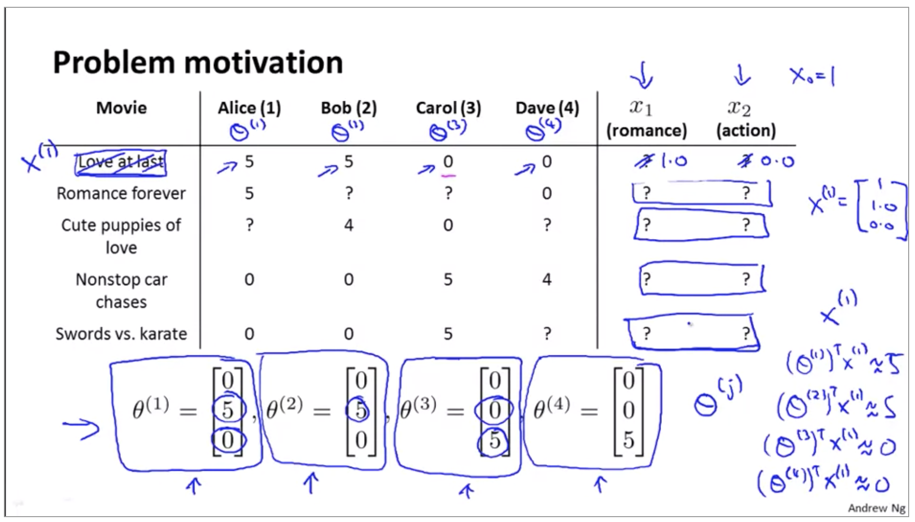
Problem Formulation
Content Based Recommendations
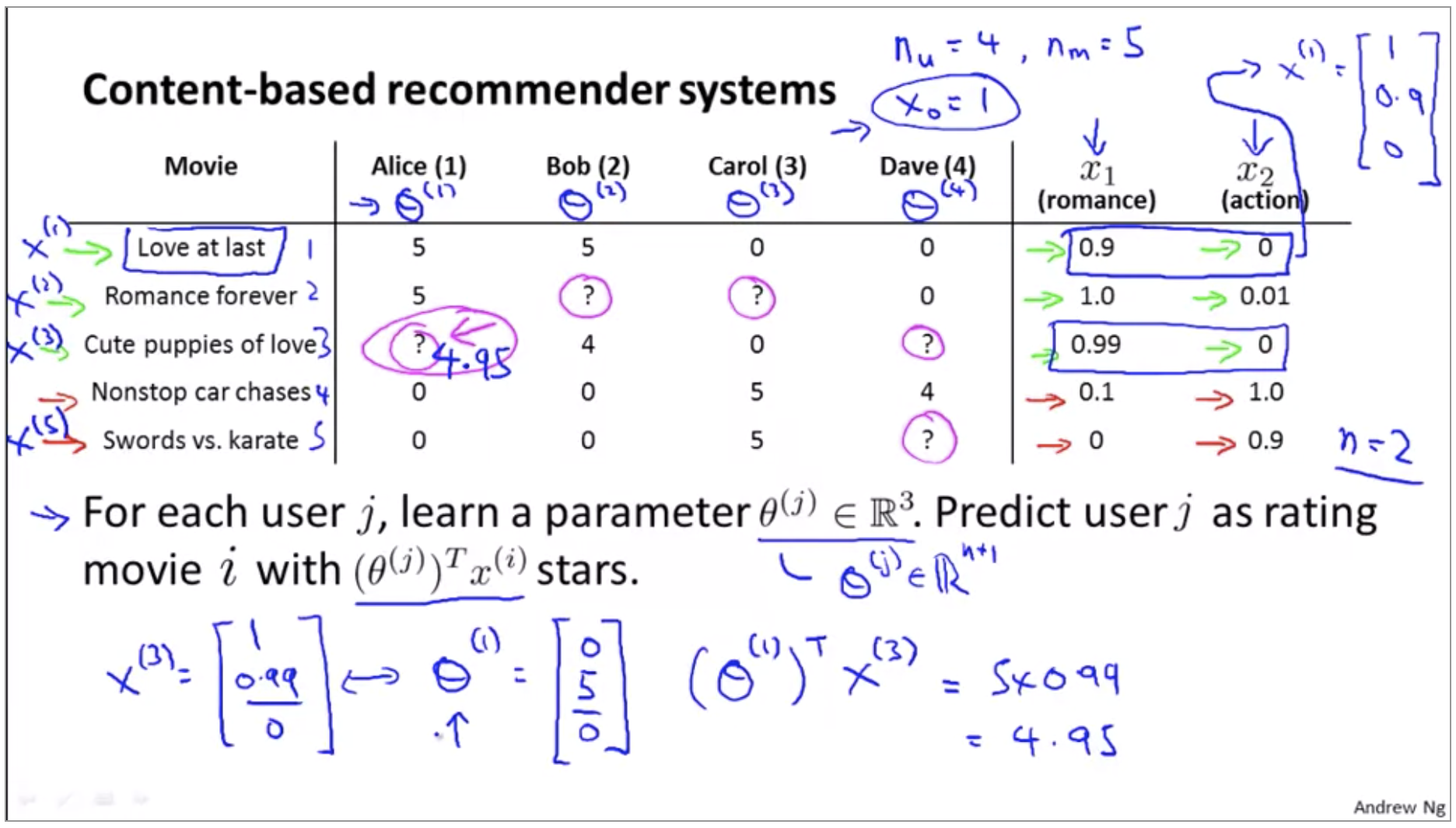
So, all we’re doing here is we’re applying a different copy of this linear regression for each user, and we’re saying that what Alice does is Alice has some parameter vector theta 1 that she uses, that we use to predict her ratings as a function of how romantic and how action packed a movie is. And Bob and Carol and Dave, each of them have a different linear function of the degree of romance and degree of action in a movie and that that’s how we’re gonna predict that their star ratings.
For user \(j\), movie \(i\), predicted rating:
\[(\theta^{(j)})^T(x^{(i)})\]To learn \(\theta^{(j)}\)(parameter for user j):
\[\min_{\theta^{(j)}} \frac{1}{2} \sum_{i:r(i,j)=1} ((\theta^{(j)})^T(x^{(i)}) - y^{(i,j)})^2 + \frac{\lambda}{2} \sum_{k=1}^n (\theta_k^{(j)})^2\]To learn \(\theta^{(1)},\theta^{(2)},...,\theta^{(n_u)}\):
\[\min_{\theta^{(1)},...,\theta^{(n_u)}} \frac{1}{2} \sum_{j=1}^{n_u} \sum_{i:r(i,j)=1} ((\theta^{(j)})^T(x^{(i)}) - y^{(i,j)})^2 + \frac{\lambda}{2} \sum_{j=1}^{n_u} \sum_{k=1}^n (\theta_k^{(j)})^2\]Gradient descent update:
\[\theta_k^{(j)} := \theta_k^{(j)} - \alpha \sum_{i:r(i,j)=1} ((\theta^{(j)})^T(x^{(i)}) - y^{(i,j)})x_k^{(i)} (\text{for } k = 0) \\ \theta_k^{(j)} := \theta_k^{(j)} - \alpha [\sum_{i:r(i,j)=1} ((\theta^{(j)})^T(x^{(i)}) - y^{(i,j)})x_k^{(i)} + \lambda\theta_k^{(j)}] (\text{for } k \neq 0)\]This particular algorithm is called a content based recommendations, or a content based approach, because we assume that we have available to us features for the different movies. And so where features that capture what is the content of these movies, of how romantic is this movie, how much action is in this movie. And we’re really using features of a content of the movies to make our predictions. But for many movies, we don’t actually have such features. Or maybe very difficult to get such features for all of our movies, for all of whatever items we’re trying to sell.
Collaborative Filtering
Collaborative filtering
Given \(\theta^{(1)}, ..., \theta^{(n_u)}\), to learn \(x^{(i)}\):
\[\min_{x^{(i)}} \frac{1}{2} \sum_{i:r(i,j)=1} ((\theta^{(j)})^T(x^{(i)}) - y^{(i,j)})^2 + \frac{\lambda}{2} \sum_{k=1}^n (x_k^{(i)})^2\]Given \(\theta^{(1)}, ..., \theta^{(n_u)}\), to learn \(x^{(1)}, ..., x^{(n_m)}\):
\[\min_{x^{(1)},...,x^{(n_m)}} \frac{1}{2} \sum_{i=1}^{n_m} \sum_{i:r(i,j)=1} ((\theta^{(j)})^T(x^{(i)}) - y^{(i,j)})^2 + \frac{\lambda}{2} \sum_{i=1}^{n_m} \sum_{k=1}^n (x_k^{(i)})^2\]So this is kind of a chicken and egg problem. Which comes first? You know, do we want if we can get the thetas, we can know the Xs. If we have the Xs, we can learn the thetas. And what you can do is, and then this actually works, what you can do is in fact randomly guess some value of the thetas.
We can sort of keep iterating, going back and forth and optimizing theta, x theta, x theta, nd this actually works and if you do this, this will actually cause your album to converge to a reasonable set of features for you movies and a reasonable set of parameters for your different users. So this is a basic collaborative filtering algorithm.
Collaborative Filtering Algorithm
Given \(x^{(1)}, ..., x^{(n_m)}\), to learn \(\theta^{(1)}, ..., \theta^{(n_u)}\):
\[\min_{\theta^{(1)},...,\theta^{(n_u)}} \frac{1}{2} \sum_{j=1}^{n_u} \sum_{i:r(i,j)=1} ((\theta^{(j)})^T(x^{(i)}) - y^{(i,j)})^2 + \frac{\lambda}{2} \sum_{j=1}^{n_u} \sum_{k=1}^n (\theta_k^{(j)})^2\]Given \(\theta^{(1)}, ..., \theta^{(n_u)}\), to learn \(x^{(1)}, ..., x^{(n_m)}\):
\[\min_{x^{(1)},...,x^{(n_m)}} \frac{1}{2} \sum_{i=1}^{n_m} \sum_{j:r(i,j)=1} ((\theta^{(j)})^T(x^{(i)}) - y^{(i,j)})^2 + \frac{\lambda}{2} \sum_{i=1}^{n_m} \sum_{k=1}^n (x_k^{(i)})^2\]Minimizing \(x^{(1)}, ..., x^{(n_m)}\) and \(\theta^{(1)}, ..., \theta^{(n_u)}\) simultaneously:
\[J(x^{(1)}, ..., x^{(n_m)},\theta^{(1)}, ..., \theta^{(n_u)}) = \frac{1}{2} \sum_{(i,j):r(i,j)=1} ((\theta^{(j)})^T(x^{(i)}) - y^{(i,j)})^2 + \frac{\lambda}{2} \sum_{i=1}^{n_m} \sum_{k=1}^n (x_k^{(i)})^2 + \frac{\lambda}{2} \sum_{j=1}^{n_u} \sum_{k=1}^n (\theta_k^{(j)})^2\]Previously we have been using this convention that we have a feature x0 equals one that corresponds to an interceptor. And the reason we do away with this convention is because we’re now learning all the features, right? So there is no need to hard code the feature that is always equal to one. Because if the algorithm really wants a feature that is always equal to 1, it can choose to learn one for itself.
Algorithm
- Initialize \(x^{(1)}, ..., x^{(n_m)}\) and \(\theta^{(1)}, ..., \theta^{(n_u)}\) to small random values(symmetry breaking).
-
Minimize \(J(x^{(1)}, ..., x^{(n_m)},\theta^{(1)}, ..., \theta^{(n_u)})\) using gradient descent (or an advanced optimization algorithm) for every \(j = 1,...n_u, i=1,...,n_m\):
\[x_k^{(i)} := x_k^{(i)} - \alpha [\sum_{j:r(i,j)=1} ((\theta^{(j)})^T(x^{(i)}) - y^{(i,j)})\theta_k^{(j)} + \lambda x_k^{(i)}] \\ \theta_k^{(j)} := \theta_k^{(j)} - \alpha [\sum_{i:r(i,j)=1} ((\theta^{(j)})^T(x^{(i)}) - y^{(i,j)})x_k^{(i)} + \lambda x_k^{(j)}]\] - For a user with parameters \(\theta\) and a movie with (learned) features \(x\), predict a star rating of \(\theta^Tx\).
Low Rank Matrix Factorization
\[Y= \begin{bmatrix} 5 & 5 & 0 & 0 \\ 5 & ? & ? & 0 \\ ? & 4 & 0 & ? \\ 0 & 0 & 5 & 4 \\ 0 & 0 & 5 & 0 \end{bmatrix}\]Predicted ratings:
\[\begin{bmatrix} (\theta^{(1)})^T(x^{(1)}) & (\theta^{(2)})^T(x^{(1)}) & ... & (\theta^{(n_u)})^T(x^{(1)}) \\ (\theta^{(1)})^T(x^{(2)}) & (\theta^{(2)})^T(x^{(2)}) & ... & (\theta^{(n_u)})^T(x^{(2)}) \\ .. & .. & .. & .. \\ (\theta^{(1)})^T(x^{(n_m)}) & (\theta^{(2)})^T(x^{(n_m)}) & ... & (\theta^{(n_u)})^T(x^{(n_m)}) \end{bmatrix}\] \[Y = X\Theta^T\]To give the collaborative filtering algorithm that you’ve been using another name. The algorithm that we’re using is also called low rank matrix factorization.
Finding related movies
For each product \(i\), we learn a feature vector \(x^{(i)} \in \R^n\).
\[x_1 = romance, x_2 = action, x_3 = comedy, x_4 = ...\]How to find movies \(j\) related to movie \(i\)?
\[\text{small:} \left\lVert x^{(i)} - x^{(j)} \right\rVert \rightarrow \text{ movie j and movie i are "similar"}\]“5 most similar movies to movie i” Find the 5 movies \(j\) with the smallest:
\[\left\lVert x^{(i)} - x^{(j)} \right\rVert\]Implementation Detail: Mean Normalization
I want to just share one last implementational detail, namely mean normalization, which can sometimes just make the algorithm work a little bit better.
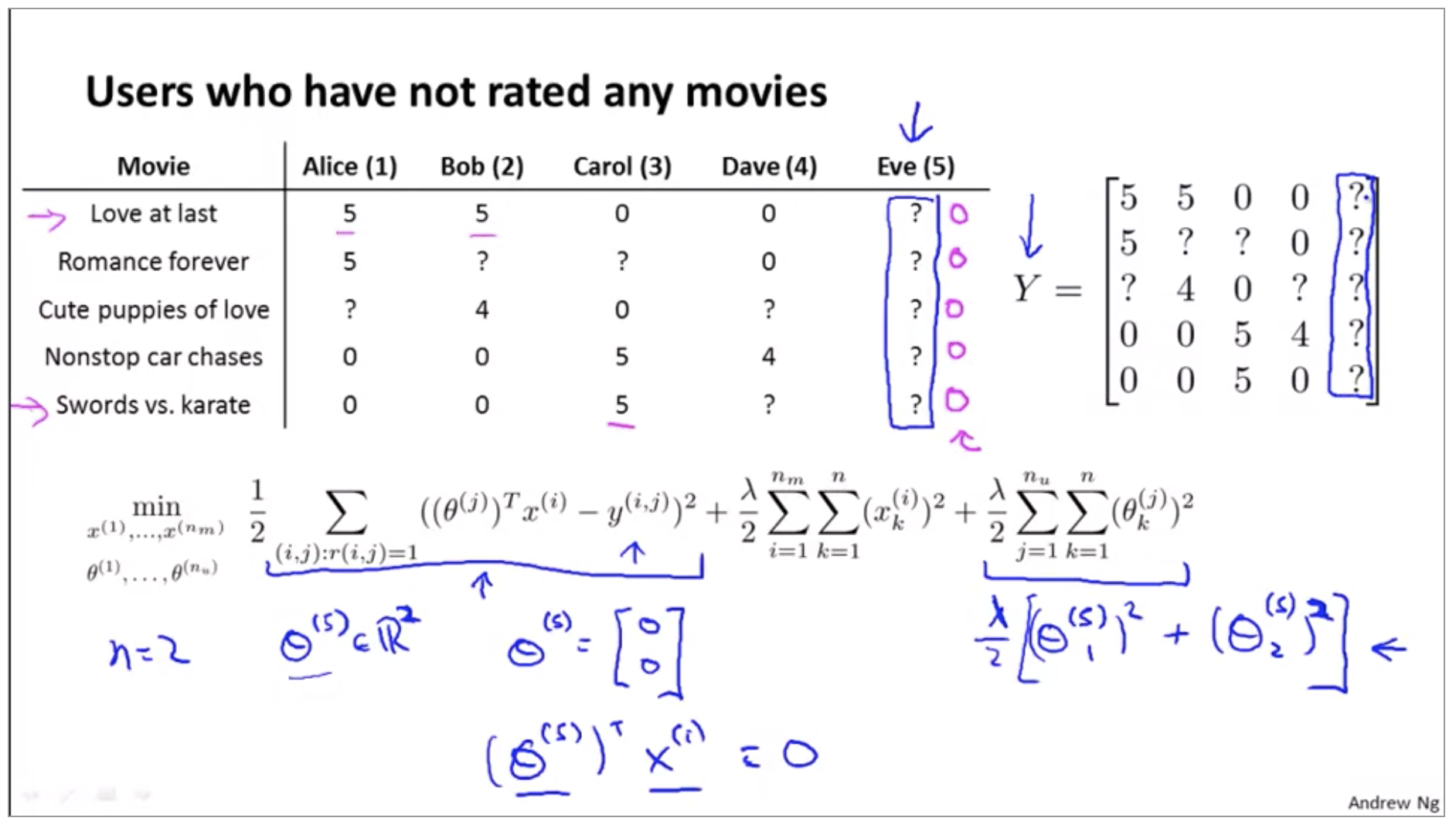
It seems not useful to just predict that Eve is going to rate everything 0 stars. And in fact if we’re predicting that eve is going to rate everything 0 stars, we also don’t have any good way of recommending any movies to her, because you know all of these movies are getting exactly the same predicted rating for Eve so there’s no one movie with a higher predicted rating that we could recommend to her, so, that’s not very good.
The idea of mean normalization will let us fix this problem. So here’s how it works.
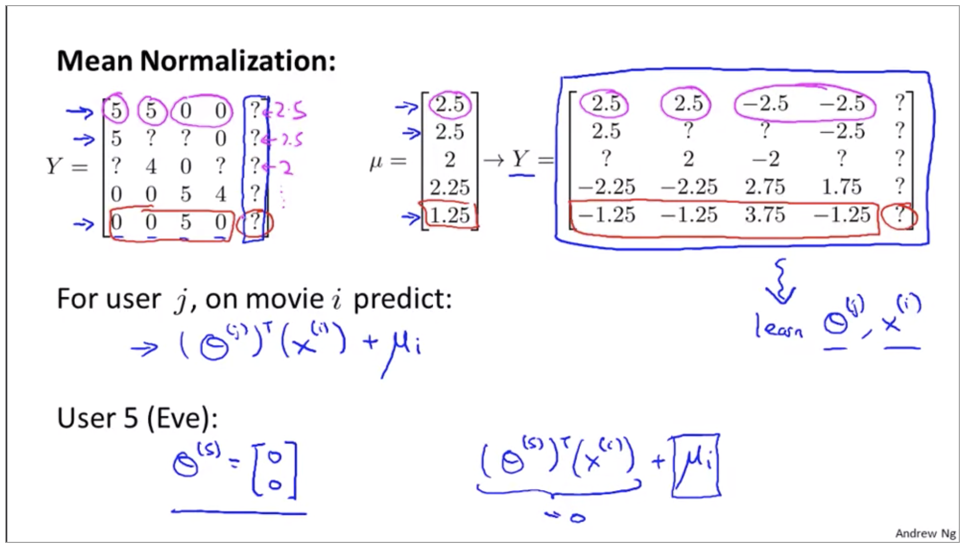
It says that if Eve hasn’t rated any movies and we just don’t know anything about this new user Eve, what we’re going to do is just predict for each of the movies, what are the average rating that those movies got.