CS229a - Week 3
Logistic Regression
Classification and Representation
Classification 예제들
- 이메일: 스팸 여부
- Online transactions: fraudulent or not(사기 여부)
- Tumor(종양): Malignant or not(악성 여부)
Binary classification problem
\[y \in \{0,1\}\]0: Negative Class, 1: Positive Class
Using Linear regression for Classification problem
\[\begin{cases} h_\theta(x) \ge 0.5 &\text{if }y=1 \\ h_\theta(x) \lt 0.5 &\text{if }y=0 \end{cases}\]- because classification is not actually a linear function
- 치우친 샘플이 Hypothesis 기울기에 영향을 주기 때문에 쓰기 어려움
Logistic Regression Model
Logistic function or Sigmoid function
Want
\[0 \le h_\theta(x) \le 1\]Equation, g = sigmoid function
\[h_\theta(x) = g(\theta^Tx) , g(z) = \frac{1}{1+e^{-z}}\] \[h_\theta(x) = \frac{1}{1+e^{-\theta^Tx}}\]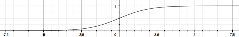
Interpretation of Hypothesis output
-
70% change of tumor being malignant
\[h_\theta(x) = 0.7\] -
probability that y = 1, given x parameterized by theta
Decision Boundary
Sigmoid function이 g의 인자가 0보다 크면 1, 0보다 작으면 0
\[h_\theta(x) = g(\theta_0 + \theta_1x_1 + \theta_2x_2)\]\(\theta_0 = -3\), \(\theta_1 = 1\), \(\theta_2 = 1\)일 때, g 함수의 인자가 0보다 크면 1
\[y = 1, -3+x_1+x_2 \ge0\]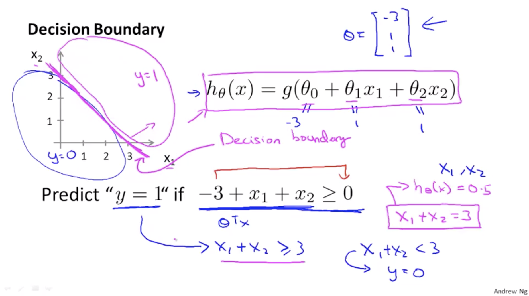
Logistic Regression Model
Cost function
Training set
\[\{(x^{(1)}, y^{(1)}), (x^{(2)}, y^{(2)}), ..., (x^{(m)}, y^{(m)}) \}\]m examples
\[x \in \begin{bmatrix} x_0 \\ x_1 \\ ... \\ x_n \end{bmatrix} x_0 = 1, y \in \{0,1\}\]Hypothesis
\[h_\theta(x) = \frac{1}{1 + e^{-\theta^Tx}}\]Cost function 일반화
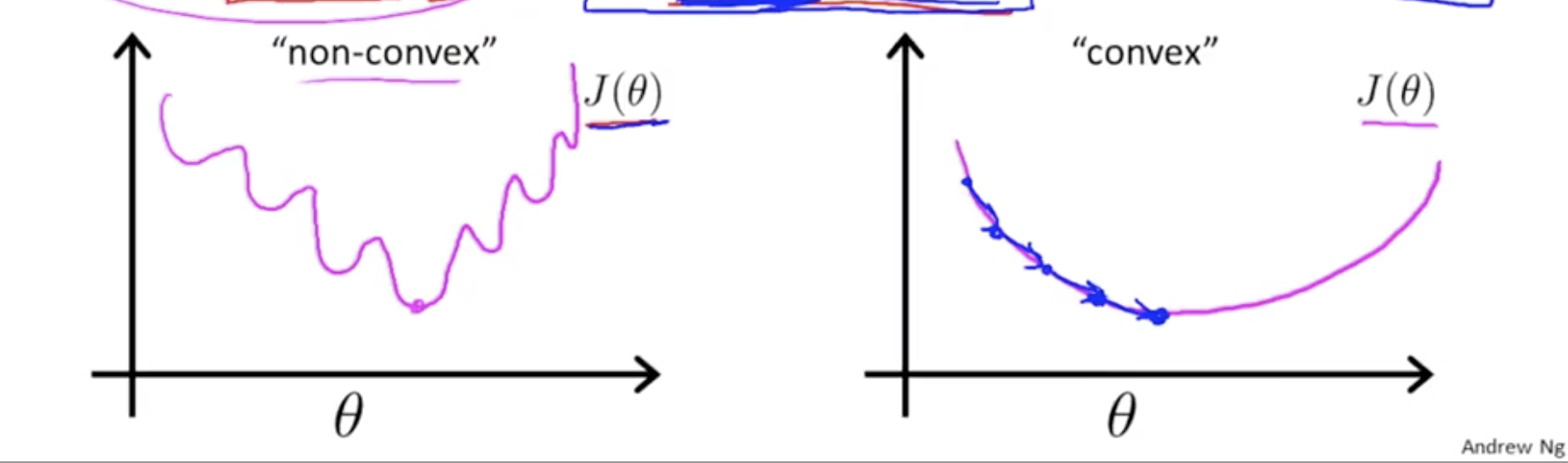
\[J(\theta) = \frac{1}{m} \sum_{i=1}^m cost(h_\theta(x^{(i)}), y^{(i)})\]Linear regression cost function
\[J(\theta) = \frac{1}{m} \sum_{i=1}^m \frac{1}{2} (h_\theta(x^{(i)}) - y^{(i)})^2\] \[Cost(h_\theta(x^{(i)}),y^{(i)}) = \frac{1}{2}(h_\theta(x^{(i)})-y^{(i)})^2\]Linear regression cost Function을 Logistic regression의 Hypothesis에 사용하면 \(J(\theta)\)가 non-convex 함수가 됨, 그래서 Local optima 도 많고 Gradient Descent를 제대로 실행할 수 없음
Logistic regression cost function
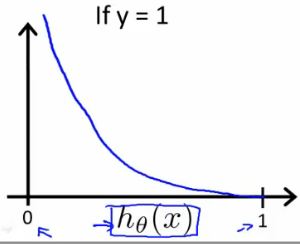
\[Cost(h_\theta(x),y) = \begin{cases} -log(h_\theta(x)) &\text{if } y=1 \\ -log(1-h_\theta(x)) &\text{if }y=0 \end{cases}\]When \(y = 1\), \(J(\theta)\) vs \(h_\theta(x)\):
When \(y = 0\), \(J(\theta)\) vs \(h_\theta(x)\):
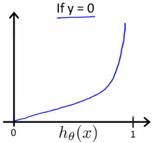
Logistic regression의 cost function은 y = 0일 때, hypothesis의 결과가 1이 나오면 cost 값이 무한대로 가고 y = 1일 때, hypothesis의 결과가 0이 나오면 cost 값이 무한대로 나옴
Simplified Cost Function and Gradient Descent
Note: y = 0 or 1 always
\[Cost(h_\theta(x),y)=-ylog(h_\theta(x)) - (1-y)log(1-h_\theta(x))\]Plugging-in the definition for full cost function
\[J(\theta) = \frac{1}{m} \sum_{i=1}^mCost(h_\theta(x^{(i)}),y^{(i)}) \\ =-\frac{1}{m}[\sum_{i=1}^m y^{(i)}log(h_\theta(x^{(i)}))+(1-y^{(i)})log(1-h_\theta(x^{(i)}))]\]Vectorized implementation:
\[J(\theta) =\frac{1}{m} \cdot (-y^Tlog(h)-(1-y)^Tlog(1-h))\]To fit parameters theta:
\[\min_\theta{J(\theta)}\]To make a prediction given new x (inference):
\[\text{Output: } h_\theta(x) = \frac{1}{1+e^{-\theta^Tx}}\]Gradient Descent, Repeat(simultaneously update all theta_j):
\[\theta_j := \theta_j - \alpha\frac{\partial}{\partial\theta_j}J(\theta)\]Calculate the derivative term, Repeat(simultaneously update all theta_j):
\[\theta_j := \theta_j -\alpha\sum_{i=1}^m(h_\theta(x^{(i)})-y^{(i)})x_j^{(i)}\]Vectorized implementation, abstract j features:
\[\theta := \theta - \alpha\frac{1}{m}\sum_{i=1}^m[h_\theta(x^{(i)})-y^{(i)}]\cdot x^{(i)}]\]XXX: 아래 식 추론 경로는 아직 모름
\[\theta := \theta - \frac{\alpha}{m}X^T(g(X\theta)-\vec{y})\]Advanced optimization
Sophisticated optimization algorithm
- Conjugate gradient, BFGS, L-BFGS
- Advantage: No need to manually pick alpha and faster than gradient descent
- 처음에는 이해하려고 하지말고 그냥 라이브러리 사용하길 권함 by Andrew Ng
- XXX: 아래 같은 분류가 있는 것 같음
- Batch gradient descent
- SGD(Stochastic Gradient Descent)
- Mini-batch gradient descent
- http://ruder.io/optimizing-gradient-descent/index.html#fn14
Linear regression Example in Octave
% costFunction
function [jVal, gradient] = costFunction(theta)

jVal = (theta(1)-5)^2 + (theta(2)-5)^2;

gradient = zeros(2,1)
gradient(1) = 2*(theta(1)-5);
gradient(2) = 2*(theta(2)-5);

% Main
options = optimset('GradObj', 'on', 'MaxIter', 100);
initialTheta = zeros(2,);

[functionVal, exitFlag] = fminunc(@costFunction, initialTheta, options)
Logistic regression Example in Octave
% costFunction
function [jVal, gradient] = costFunction(theta)

jVal = % code to compute J(theta)
gradient(1) = % derivative for theta_0, CODE#1
gradient(2) = % derivative for theta_1, CODE#2
CODE#1
\[\frac{1}{m}\sum_{i=1}^m[h_\theta(x^{(i)}-y^{(i)}) \cdot x_0^{(i)}](=\frac{\partial}{\partial\theta_0}J(\theta))\]Multi-class Classification(one-vs-all)
- 이메일 Tagging: 직장, 친구, 가족, 취미
- 날씨: Sunny, Cloudy, Rain, Snow
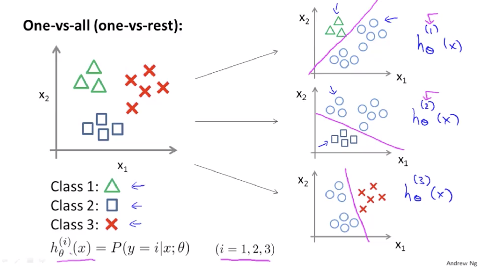
One-vs-all: Train a logistic regression classifier \(h_\theta^{(i)}(x)\) for each class i
Inference, pick the class i that maximizes:
\[\max_ih_\theta^{(i)}(x)\]Regularization
The Problem of Overfitting
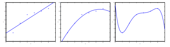
- Under-fitting, High bias
- the algorithm has a very strong preconception
- hypothesis function maps poorly to the trend of the data
- It is usually caused by a function that is too simple or uses too few features
- Just-right
- Over-fitting, High variance: We don’t have enough data to constrain it
- We have too many features, the learned hypothesis may fit the training set very well, but fail to generalize to new examples
Addressing over-fitting
- plotting the data: feature가 많은 경우 시각적으로 표현하기 어려움
- 1) Reduce number of features
- Manually select which features to keep
- Model selection algorithm(뒤에 나옴)
- 2) Regularization(정규화)
- Keep all the features, but reduce magnitude/ values of parameters \(\theta_j\)
- Works well when we have a lot of features, each of which contributes a bit to predicting y
Cost function
High order degree polynomial, Suppose we penalize and make \(\theta_3\), \(\theta_4\) really small
\[\min_\theta\frac{1}{2m}\sum_{i=1}^m(h_\theta(x^{(i)})-y^{(i)})^2+1000 \cdot \theta_3^2 +1000 \cdot \theta_4^2\]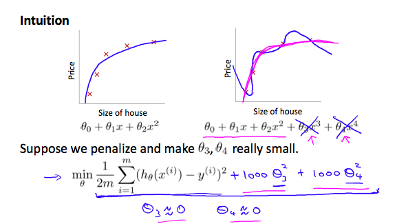
Regularization: penalize the parameter values being large
- “Simpler” hypothesis
- Less prone to overfitting
- Don’t penalize \(\theta_0\)
Regularization example: Housing problem with Linear regression
\[\text{Features: } x_1,x_2,...,x_{100}\\ \text{Parameters: }: \theta_0,\theta_1,...,\theta_{100}\]Add regularization term at the end of Cost function:
\[J(\theta) = \frac{1}{2m} [\sum_{i=1}^m(h_\theta(x^{(i)})-y^{(i)})^2 + \lambda\sum_{j=1}^n\theta_j^2]\]- regularization parameter: \(\lambda\)
- It determines how much the costs of our theta parameters are inflated
- If \lambda is set to an extremely large value, the algorithm results in under-fitting
Regularized linear regression
Gradient descent, Repeat until convergence:
\[\theta_j := \theta_j - \alpha[\frac{1}{m} \sum_{i=1}^m(h_\theta(x^{(i)})-y^{(i)})x_j^{(i)} + \frac{\lambda}{m}\theta_j]\] \[\theta_j := \theta_j(1-\alpha\frac{\lambda}{m}) - \alpha\frac{1}{m} \sum_{i=1}^m(h_\theta(x^{(i)})-y^{(i)})x_j^{(i)}\]First term: learning rate and lambda is small it’s value is less than 1(i.g. 0.99)
\[\theta_j(1-\alpha\frac{\lambda}{m})\]Normal equation
\[X = \begin{bmatrix} (x^{(1)})^T \\ ... \\ (x^{(m)})^T \end{bmatrix}, y = \begin{bmatrix} y^{(1)} \\ ... \\ y^{(m)} \end{bmatrix}\] \[\min_\theta J(\theta)\]If \(\lambda > 0\),
\[\Theta = (X^TX+\lambda\begin{bmatrix} 0 & 0 & 0 & 0\\ 0 & 1 & 0 & 0 \\ 0 & 0 & ... & 0\\ 0 & 0 & 0 & 1 \end{bmatrix})^{-1}X^Ty\]Using regularization also takes care of any non-invertibility issues of the X transpose X matrix as well
Regularized logistic regression
Over-fitting logistic regression
\[h_\theta(x) = g(\theta_0 + \theta_1x_1 + \theta_2x_1^2 + \theta_3x_1^2x_2 + \theta_4x_1^2x_2^2 + \theta_5x_1^2x_2^3+ ...)\]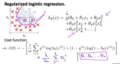
Gradient descent, Repeat(linear regression과 모양은 비슷하지만, hypothesis가 다름):
\[\theta_0 := \theta_0 - \alpha[\frac{1}{m} \sum_{i=1}^m(h_\theta(x^{(i)})-y^{(i)})x_0^{(i)}] \\ \theta_j := \theta_j - \alpha[\frac{1}{m} \sum_{i=1}^m(h_\theta(x^{(i)})-y^{(i)})x_j^{(i)} + \frac{\lambda}{m}\theta_j],(j=1,2,3,...,n)\]Apply Advanced optimization
function [jVal, gradient] = costFunction(theta)
  jVal = % code to compute J(theta)

  gradient(1) = % code to compute partial theta_0 of J(theta)
  gradient(n + 1) = % code to compute partial theta_n of J(theta)
jVal:
\[J(\theta) = -\frac{1}{m}\sum_{i=1}^m[y^{(i)}log(h_\theta(x^{(i)}))+(1-y^{(i)})log(1-h_\theta(x^{(i)}))] + \frac{\lambda}{2m}\sum_{j=1}^n\theta_j^2\]gradient(1):
\[\frac{1}{m}\sum_{i=1}^m(h_\theta(x^{(i)})-y^{(i)})x_0^{(i)}\]gradient(n+1):
\[\frac{1}{m}\sum_{i=1}^m(h_\theta(x^{(i)})-y^{(i)})x_n^{(i)} + \frac{\lambda}{m}\theta_n\]You probably know quite a lot more machine learning right now than frankly, many of the Silicon Valley engineers out there having very successful careers. You know, making tons of money for the companies. Or building products using machine learning algorithms. So, congratulations. - Andrew Ng
XXX: Andrew Ng는 강의에서 묘한 웃음으로 말했는데, 뭘 의미하는 걸까?
XXX: Week 3 Programming 숙제에서는 Sigmoid Function, Cost Function, Predict 구현 했음. 이전처럼 Gradient Descent는 직접 구현하지 않고 Octave에 있는 fminunc를 사용했다. 수식에 맞게 Vector와 Matrix를 잘 조립하는게 중요했는데, size 함수로 하나씩 찍어보면서 맞춰야 했다.
%  Set options for fminunc
options = optimset('GradObj', 'on', 'MaxIter', 400);

%  Run fminunc to obtain the optimal theta
%  This function will return theta and the cost
[theta, cost] = ...
  fminunc(@(t)(costFunction(t, X, y)), initial_theta, options);