CS229a - Week 8

Written by hackerwins on July 10, 2019

In unsupervised learning what we do is we give this sort of unlabeled training set to an algorithm and we just ask the algorithm find some structure in the data for us.

Clustering

So, what is clustering good for? Early in this class I already mentioned a few applications.

One is market segmentation where you may have a database of customers and want to group them into different marker segments so you can sell to them separately or serve your different market segments better.
Social network analysis. There are actually groups have done this things like looking at a group of people’s social networks. So, things like Facebook, Google+, or maybe information about who other people that you email the most frequently and who are the people that they email the most frequently and to find coherence in groups of people. So, this would be another maybe clustering algorithm where you know want to find who are the coherent groups of friends in the social network?
Using clustering to organize computer clusters or to organize data centers better. Because if you know which computers in the data center in the cluster tend to work together, you can use that to reorganize your resources and how you layout the network and how you design your data center communications.
Using clustering algorithms to understand galaxy formation and using that to understand astronomical data.

K-means algorithm

The first step is to randomly initialize two points, called the cluster centroids. So, these two crosses here, these are called the Cluster Centroids K Means is an iterative algorithm and it does two things. First is a cluster assignment step, and second is a move centroid step. So, let me tell you what those things mean.

Input:

\(K\)(number of clusters)
Training set
\[\{x^{(1)},x^{(2)},...,x^{(m)}\} \\ x^{(i)} \in \R^n \text{(drop } x_0 = 1\text{ convention)}\]
centroids
\[\mu_1,\mu_2,...,\mu_k \in \R^n\]

Algorithem:

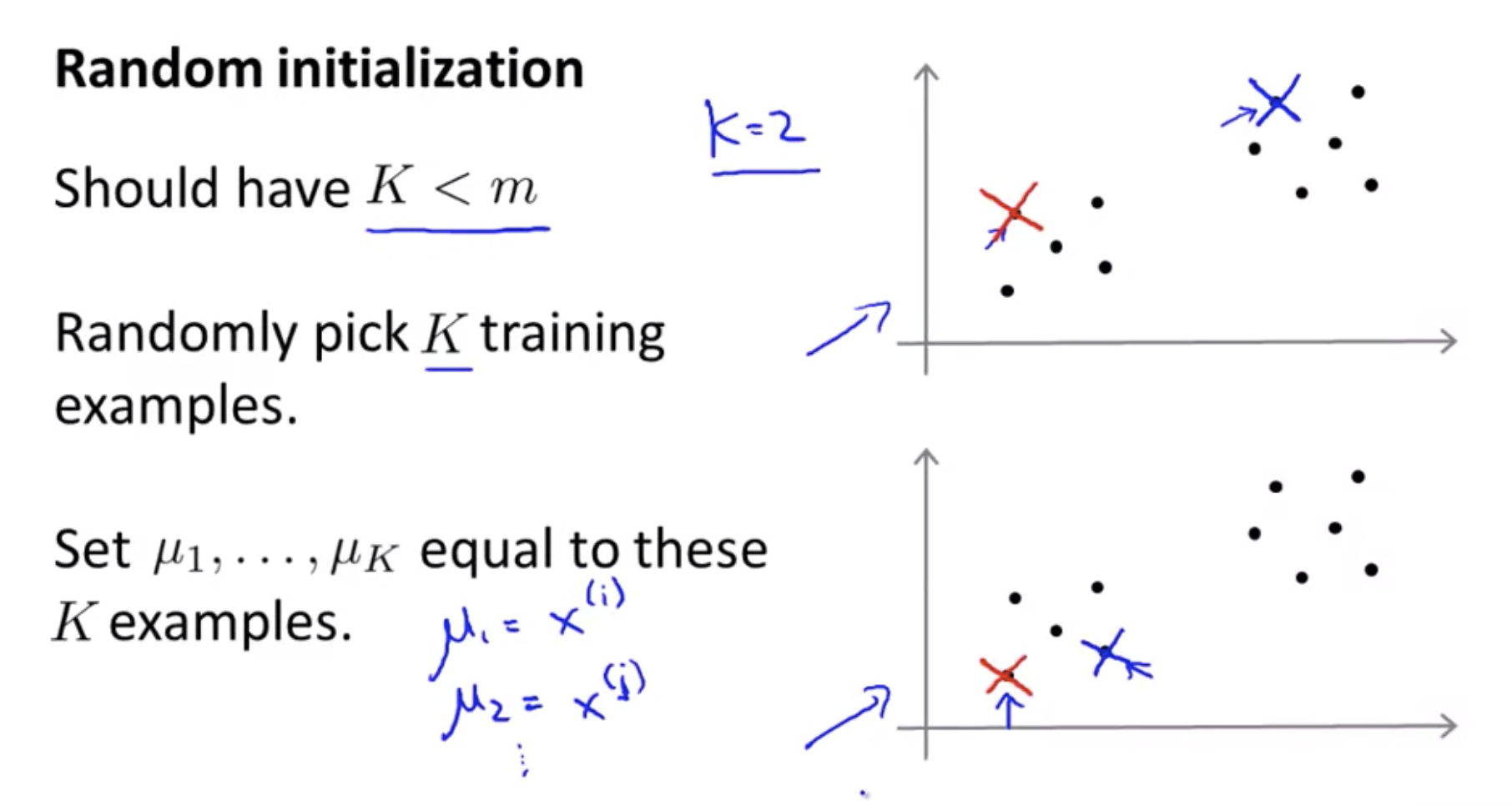
Randomly initialize K cluster centroids \mu_1, \mu_2, ..., \mu_K \in \R^n
Repeat {
  // Cluster assignment step
  for i = 1 to m
    c^{(i)} := index(from 1 to K) of cluster centroid closest to x ^{(i)}
  // Move centroid step
  for k = 1 to K
    u_k := average(mean) of points assigned to cluster k
}

Cluster assignment step

\[c^{(i)} = \min_k \left\lVert x^{(i)} - \mu_k \right\rVert^2\]

Move centroid step

\[x^{(1)},x^{(5)},x^{(6)},x^{(10)} \rightarrow c^{(1)}=2,c^{(5)}=2,c^{(6)}=2,c^{(10)}=2 \\ \mu_2 = \frac{1}{4}[x^{(1)},x^{(5)},x^{(6)},x^{(10)}] \in R^n\]

K-means for non-separated clusters

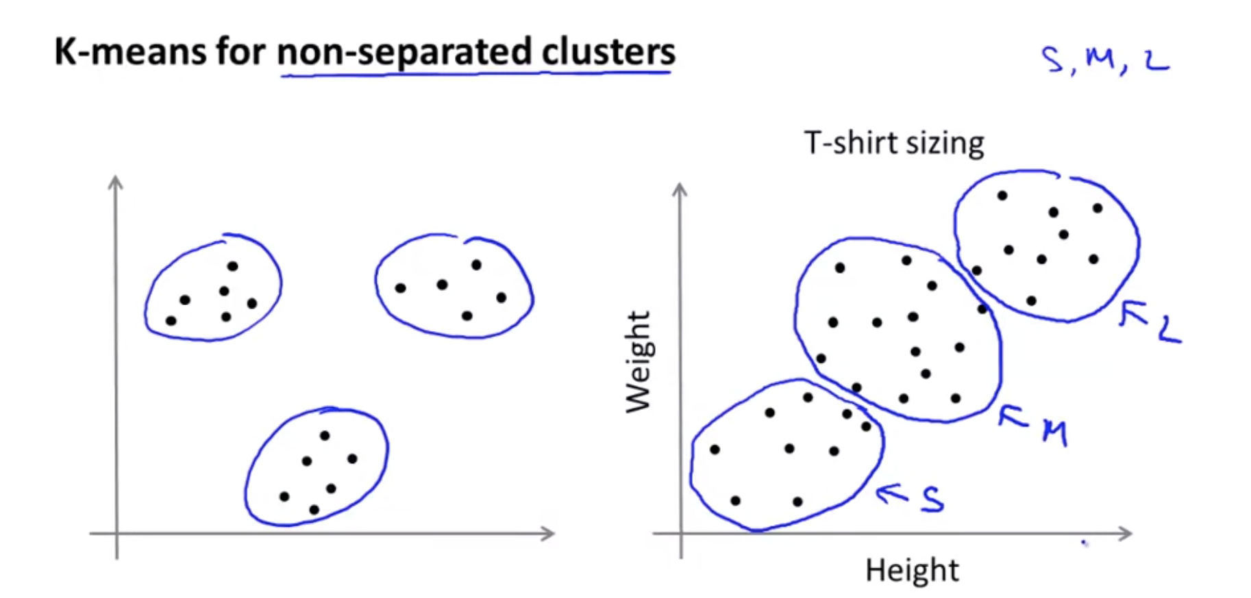
Even though the data, you know, before hand it didn’t seem like we had 3 well separated clusters, K Means will kind of separate out the data into multiple pluses for you.

Clustering: Optimization objective

It turns out that k-means also has an optimization objective or a cost function that it’s trying to minimize.

Knowing what is the optimization objective of k-means will help us to debug the learning algorithm and just make sure that k-means is running correctly.
How we can use this to help k-means find better costs for this and avoid the local optima.

Notations

\(c^{(i)}\) = index of cluster (\(1,2,...,K\)) to which example \(x^{(i)}\) is currently assigned
\(\mu_k\) = clutser centroid k (\(\mu_k \in \R^n\))
\(\mu_{c^{(i)}}\) = cluster centroid of cluster to which example \(x^{(i)}\) has been assgiend

\[x^{(i)} \rightarrow 5, c^{(i)}=5 \\ \mu_{c^{(i)}} = \mu_5\]

Optimization objective:

\[J(c^{(1)},...,c^{(m)},\mu_1,...,\mu_K)=\frac{1}{m}\sum_{i=1}^m \left\lVert x^{(i)} - \mu_{c^{(i)}} \right\rVert^2\] \[\min_{c^{(1)},...c^{(m)}, \mu_1, ..., \mu_K} J(c^{(1)},...c^{(m)},\mu_1,...,\mu_K)\]

This cost function is sometimes also called the distortion cost function.

XXX: https://en.wikipedia.org/wiki/Distortion_function

Clustering: Random intialization

These local optima correspond to is really solutions where K-means has gotten stuck to the local optima and it’s not doing a very good job minimizing this distortion function J.

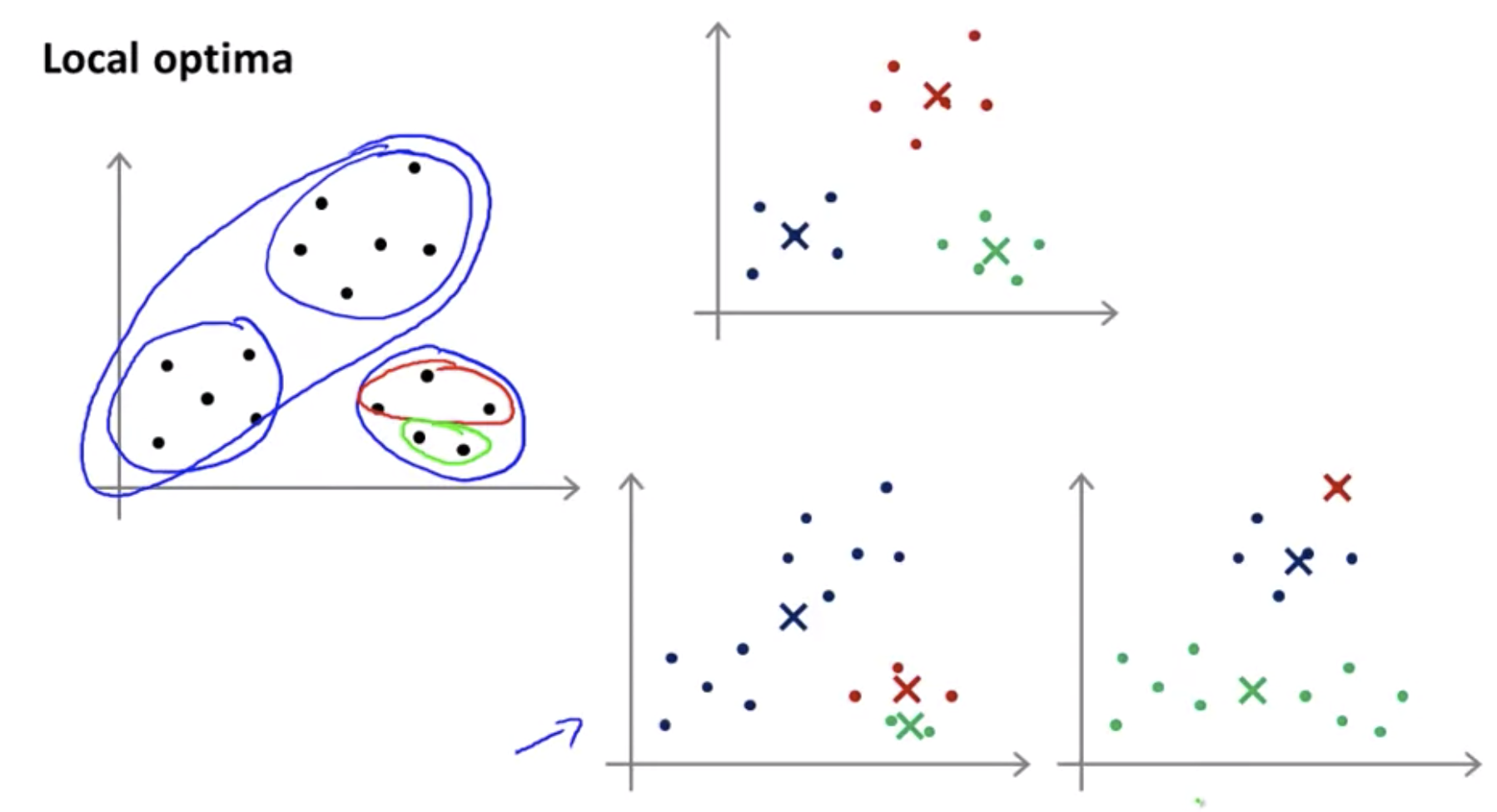
To avoid local optima, try multiple random initialization(50 ~ 1000).

for i = 1 to 100 {
  Randomly initialize K-means.
  Run K-means. Get c^{(1)}, ..., c^{(m)},\mu_1, ..., \mu_K
  Compute cost function(distortion), J(c^{(m)},\mu_1, ..., \mu_K)
}

If you’re trying to learn a clustering with a relatively small number of clusters, 2, 3, 4, 5, maybe, 6, 7, using multiple random initializations can sometimes, help you find much better clustering of the data. But, even if you are learning a large number of clusters, the initialization, the random initialization method that I describe here. That should give K-means a reasonable starting point to start from for finding a good set of clusters.

Clustering: Choosing the Number of clusters

There actually isn’t a great way of answering this or doing this automatically and by far the most common way of choosing the number of clusters, is still choosing it manually by looking at visualizations or by looking at the output of the clustering algorithm or something else.

Elbow method:

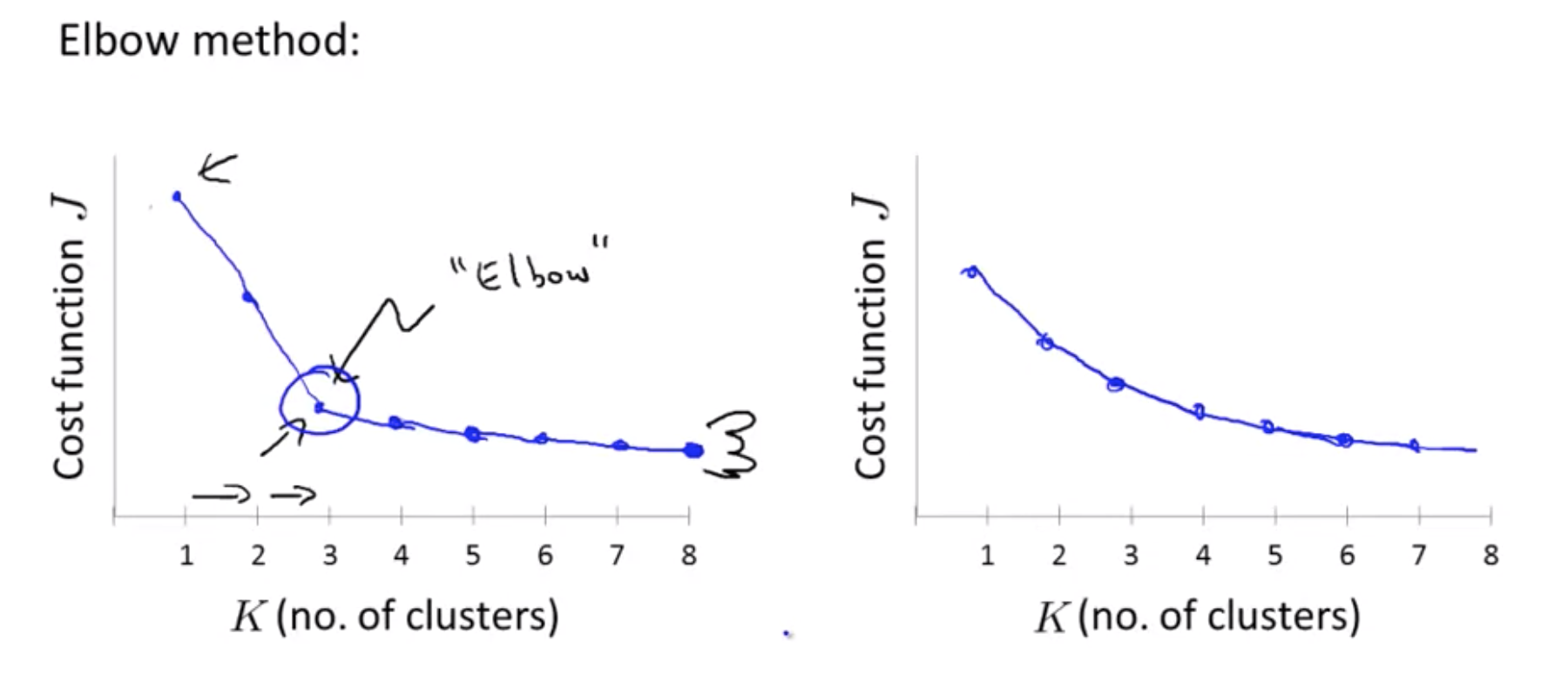
So, just summarize, for the most part, the number of customers K is still chosen by hand by human input or human insight. One way to try to do so is to use the Elbow Method, but I wouldn’t always expect that to work well, but I think the better way to think about how to choose the number of clusters is to ask, for what purpose are you running K-means? And then to think, what is the number of clusters K that serves that, you know, whatever later purpose that you actually run the K-means for.

Dimensionality Reduction

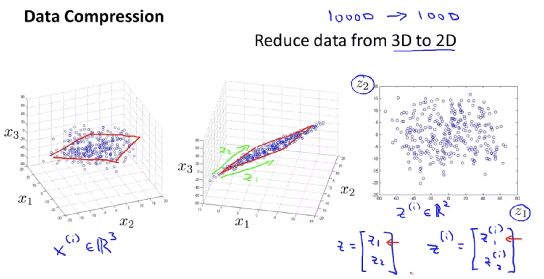
Data compression

There are a couple of different reasons why one might want to do dimensionality reduction. One is data compression, and as we’ll see later, a few videos later, data compression not only allows us to compress the data and have it therefore use up less computer memory or disk space, but it will also allow us to speed up our learning algorithms.

If you have hundreds or thousands of features, it is often this easy to lose track of exactly what features you have.

Data Visualization

How do you visualize this data? If you have 50 features, it’s very difficult to plot 50-dimensional data. you can do is reduce the data from 50 D, from 50 dimensions to 2D, so you can plot this as a 2 dimensional plot.

\[x^i \in \R^{50} \rightarrow z^{(i)} \in \R^k\]

PCA(Principal Component Analysis) problem formulation

So what PCA does formally is it tries to find a lower dimensional surface, really a line in this case, onto which to project the data so that the sum of squares of these little blue line segments is minimized. The length of those blue line segments, that’s sometimes also called the projection error. As an aside, before applying PCA, it’s standard practice to first perform mean normalization at feature scaling.

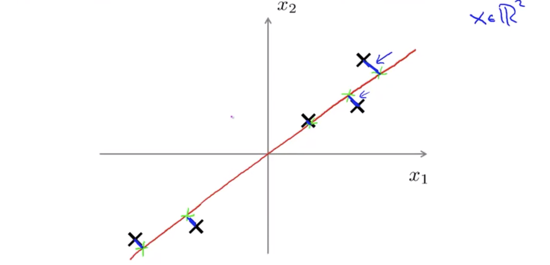
Reduce from n-dimension to k-dimension: Find k vectors \(u^{(1)}, u^{(2)}, ..., u^{(k)}\) onto which to project the data so as to minimize the projection error.

XXX: https://en.wikipedia.org/wiki/Linear_subspace

PCA is not linear regression

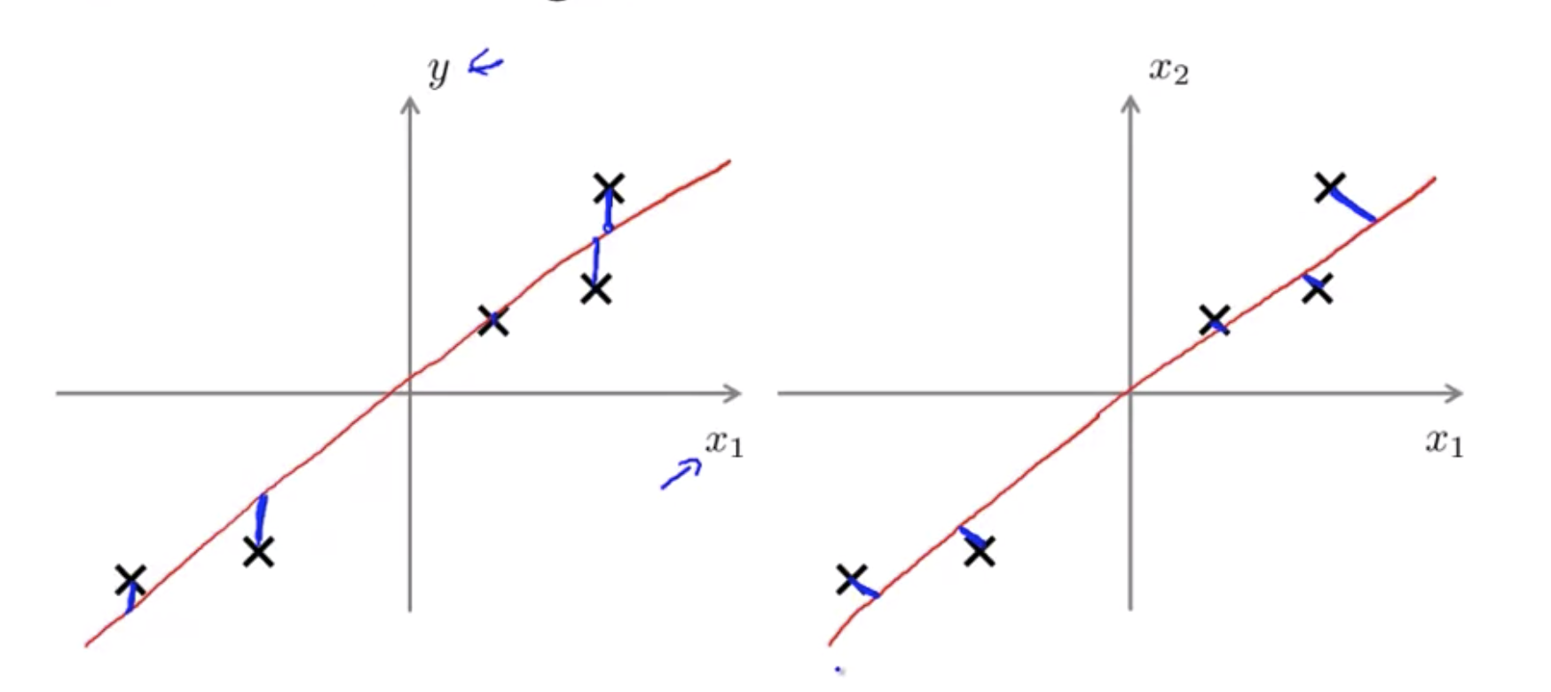
Linear regression as well as taking all the values of x and try to use that to predict y. Whereas in PCA, there is no distinguish, or there is no special variable y that we’re trying to predict. And instead, we have a list of features, \(x_1, x_2\), and so on, up to \(x_n\), and all of these features are treated equally, so no one of them is special.

PCA algorithm

Reduce data from n-dimensions to k-dimensions

Compute “covariance matrix”:

\[\Sigma = \frac{1}{m} \sum_{i=1}^n (x^{(i)})(x^{(i)})^T\]

Compute “eigenvector” of matrix \(\Sigma\):

Sigma = (1 / m) * (X' * X);
[U,S,V] = svd(Sigma); // U: n x n matrix
Ureduce = U(:, 1:k);
z = Ureduce' * X;

From [U,S,V] = svd(Sigma), we get:

\[U = \begin{bmatrix} | & | & ... & | \\ u^{(1)} & u^{(2)} & ... & u^{(n)} \\ | & | & ... & | \end{bmatrix}\] \[x\in\R^n \rightarrow z \in \R^k\] \[z = \begin{bmatrix} | & | & ... & | \\ u^{(1)} & u^{(2)} & ... & u^{(k)} \\ | & | & ... & | \end{bmatrix}^T x, z_j =(u^{(j)})^Tx\]

Okay, that was probably much more linear algebra than you needed to know. In case none of that made sense, don’t worry about it. All you need to know is that this system command you should implement in Octave.

XXX: 본 내용 같아서 찾아보니 이전에 얼굴 인식 코딩할 때 Eigenface 만들 때 사용했음

Reconstruction from compressed representation

\[z = U_{reduced}^Tx \\ X_{approx} = U_{reduce}z, \text{ } (U_{reduce} \in \R^{n\times k}, z \in \R^{k \times 1})\]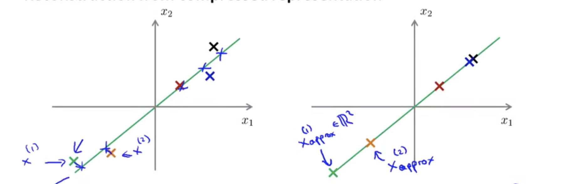

Choosing the Number of principal components

This number K is also called the number of principle components or the number of principle components that we’ve retained.

Average squared projection error:

\[\frac{1}{m} \sum_{i=1}^m \left\lVert x^{(i)} - x_{approx}^{(i)} \right\rVert^2\]

Total variation in the data(On average, how far are training examples from the origin):

\[\frac{1}{m}\sum_{i=1}^m \left\lVert x^{(i)} \right\rVert^2\]

Typically, choose k to be smallest value so that(i.g. “99% of variance is retained”):

\[\frac{\frac{1}{m} \sum_{i=1}^m \left\lVert x^{(i)} - x_{approx}^{(i)} \right\rVert^2}{\frac{1}{m}\sum_{i=1}^m \left\lVert x^{(i)} \right\rVert^2} \le 0.01\]

Fortunately when you implement PCA it actually, in this step, it actually gives us a quantity that makes it much easier to compute these things as well.

[U,S,V] = svd(Sigma) // S is a diagonal matrix.

\[1 - \frac{\sum_{i=1}^ks_{ii}}{\sum_{i=1}^ns_{ii}} = \frac{\frac{1}{m} \sum_{i=1}^m \left\lVert x^{(i)} - x_{approx}^{(i)} \right\rVert^2}{\frac{1}{m}\sum_{i=1}^m \left\lVert x^{(i)} \right\rVert^2}\]

Advice for applying PCA

Supervised learning speedup

\[x^{(1)},x^{(2)},...,x^{(m)} \in \R^{10000} \\ \downarrow \text{ } \\ z^{(1)},z^{(2)},...,z^{(m)} \in \R^{1000}\]

New training set:

\[(z^{(1)},y^{(1)}),(z^{(2)},y^{(2)}),...,(z^{(m)},y^{(m)})\]

Note: mapping \(x^{(i)} \rightarrow y^{(i)}\) should be defined by running PCA only on the training set. This mapping can be applied as well to the examples in the cross validation and test sets.

Bad use of PCA: To prevent overfitting

If you want to use this method to reduce the dimensional data, to try to prevent over-fitting, it might actually work OK. But this just is not a good way to address over-fitting and instead, if you’re worried about over-fitting, there is a much better way to address it, to use regularization instead of using PCA to reduce the dimension of the data.

PCA is sometimes used where it shouldn’t be

How about doing the whole thing without using PCA? Before implementing PCA, first try running what every you want to do with the original/raw data. Only if that doesn’t do what you want, then implement PCA.

XXX: “Premature Optimization Is the Root of All Evil” 과 같은 맥락 같음

← → Top