DLS Course 1 - Week 2
Logistic Regression as a Neural Network
Binary Classification
Logistic regression is an algorithm for binary classification.
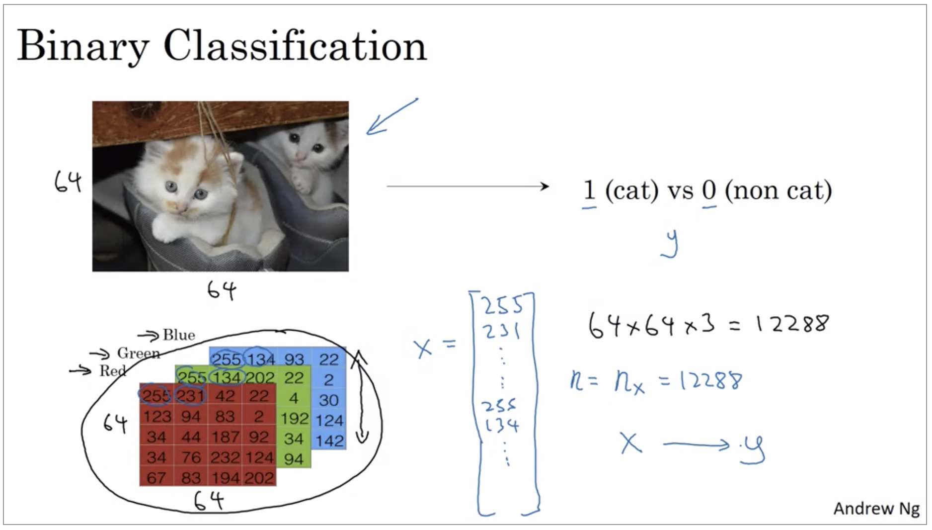
Here’s an example of a binary classification problem. You might have an input of an image, like that, and want to output a label to recognize this image as either being a cat, in which case you output 1, or not-cat in which case you output 0.
To store an image your computer stores three separate matrices corresponding to the red, green, and blue color channels of this image. So if your input image is 64 pixels by 64 pixels, then you would have 3 64 by 64 matrices corresponding to the red, green and blue pixel intensity values for your images. So to turn these pixel intensity values into a feature vector, what we’re going to do is unroll all of these pixel values into an input feature vector x. If this image is a 64 by 64 image, the total dimension of this vector x will be 64 by 64 by 3 because that’s the total numbers we have in all of these matrixes.
Notation
Single train example:
\[(x,y) \text{ } x \in\R^n, y\in \{0,1\}\]Training set:
\[\{(x^{(1)}, y^{(1)}), (x^{(2)}, y^{(2)}), ... (x^{(m)}, y^{(m)})\}\]Training set:
\[M_{train}, M_{test}\]Matrix X(group the training examples input x into matrix):
\[X \in \R^{n_x \times m}\]Output:
\[Y = \begin{bmatrix} y^{(1)} & y^{(2)} & ... & y^{(m)} \end{bmatrix} \\ Y \in \R^{1 \times m}\]Logistic Regression
We’ll go over logistic regression. This is a learning algorithm that you use when the output labels Y in a supervised learning problem are all either zero or one, so for binary classification problems.
\[\text{Given } x, \text{ want } \hat{y} = P(y=1|x)\]input vector:
\[x \in \R^{n_x}\]parameters:
\[w \in \R^{n_x}, b \in \R\]Output:
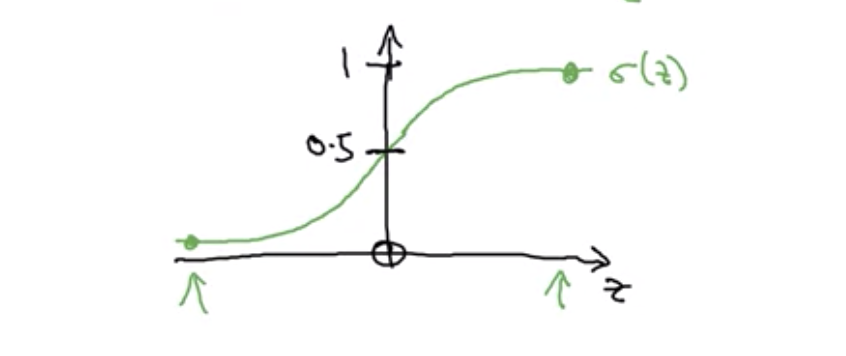
\[\hat{y} = \sigma(w^Tx + b)\]So Y hat should really be between zero and one, and it’s difficult to enforce that because W transpose X plus B can be much bigger than one or it can even be negative, which doesn’t make sense for probability. So in logistic regression, our output is instead going to be Y hat equals the sigmoid function applied to this quantity.
When we programmed neural networks, we’ll usually keep the parameter W and parameter B separate.
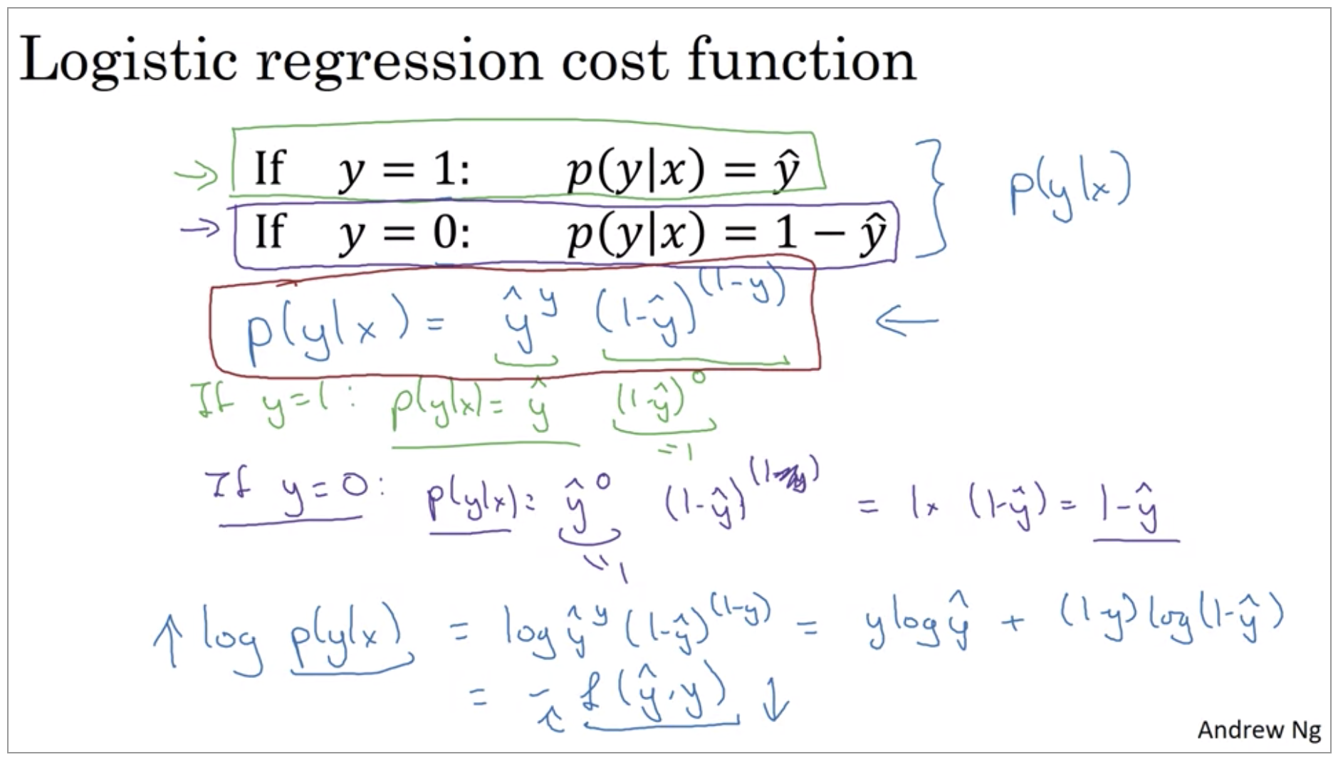
Logistic Regression Cost Function
The superscript parentheses i refers to data, be it. X or Y or Z or something else associated with the i-th training example.
\[\hat{y} = \sigma(w^Tx + b), \text{where } \sigma(z) = \frac{1}{1+e^{-z}}\] \[\text{Given } \{(x^{(1)}, y^{(1)}), ... (x^{(m)}, y^{(m)})\}, \text{ want } \hat{y}^{(i)} \approx y^{(i)}\]Loss function is a function you’ll need to define to measure how good our output y-hat is when the true label is y. One thing you could do is define the loss when your algorithm outputs y-hat and the true label as Y to be maybe the square error or one half a square error. It turns out that you could do this, but in logistic regression people don’t usually do this because when you come to learn the parameters, you find that the optimization problem which we talk about later becomes non-convex. So you end up with optimization problem with multiple local optima.
Loss(error) function:
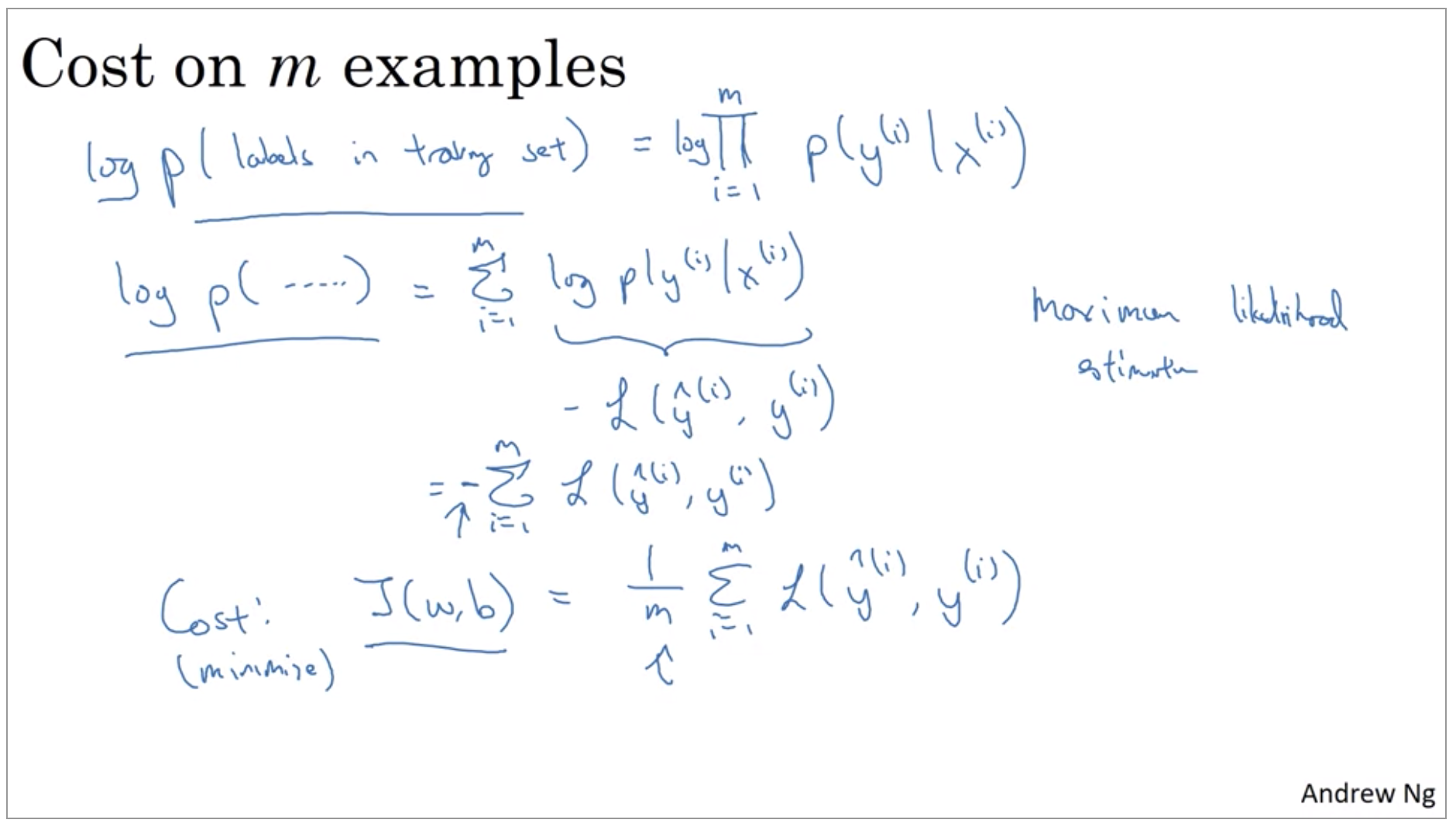
\[L(\hat{y},y) = -(ylog\hat{y} + (1-y)log(1-\hat{y}))\]Cost function:
\[J(w,b) = \frac{1}{m}\sum_{i=1}^m L(\hat{y}^{(i)}, y^{(i)}) = \frac{1}{m}\sum_{i=1}^m[-(y^{(i)}log\hat{y}^{(i)} + (1-y^{(i)})log(1-\hat{y}^{(i)}))]\]So the terminology I’m going to use is that the loss function is applied to just a single training example like so. And the cost function is the cost of your parameters. So in training your logistic regression model, we’re going to try to find parameters W and B that minimize the overall costs function J.
It turns out that logistic regression can be viewed as a very very small neural network.
Gradient Descent
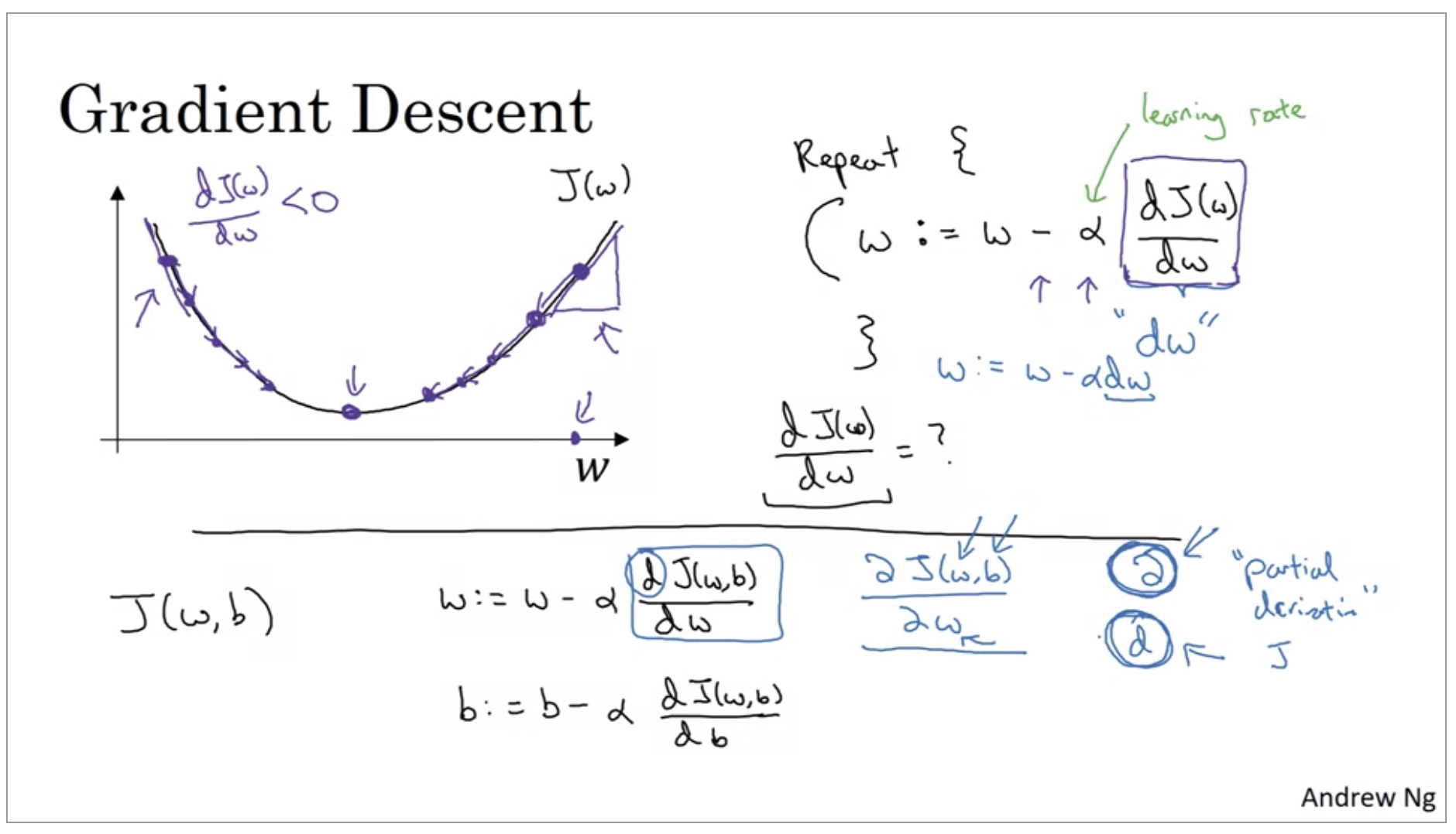
It turns out that the cost function J is a convex function. So the fact that our cost function J(w,b) is convex is one of the huge reasons why we use this particular cost function, J, for logistic regression. So to find a good value for the parameters, what we’ll do is initialize w and b to some initial value. And for logistic regression almost any initialization method works, usually you initialize the value to zero. Random initialization also works, but people don’t usually do that for logistic regression. Because this function is convex, no matter where you initialize, you should get to the same point or roughly the same point.
And what gradient descent does is it starts at that initial point and then takes a step in the steepest downhill direction.
Derivatives
If I nudge a to the right a little bit, I expect f(a) to go up by three times as much as I nudged the value of little a. Talking about what happens if we nudged the variable a by 0.001.
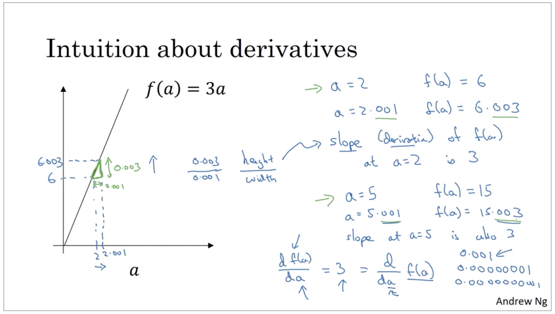
Now, one property of the derivative is that, no matter where you take the slope of this function, it is equal to three, whether a is equal to two or a is equal to five. The slope of this function is equal to three, meaning that whatever is the value of a, if you increase it by 0.001, the value of f of a goes up by three times as much.
More Derivative Examples
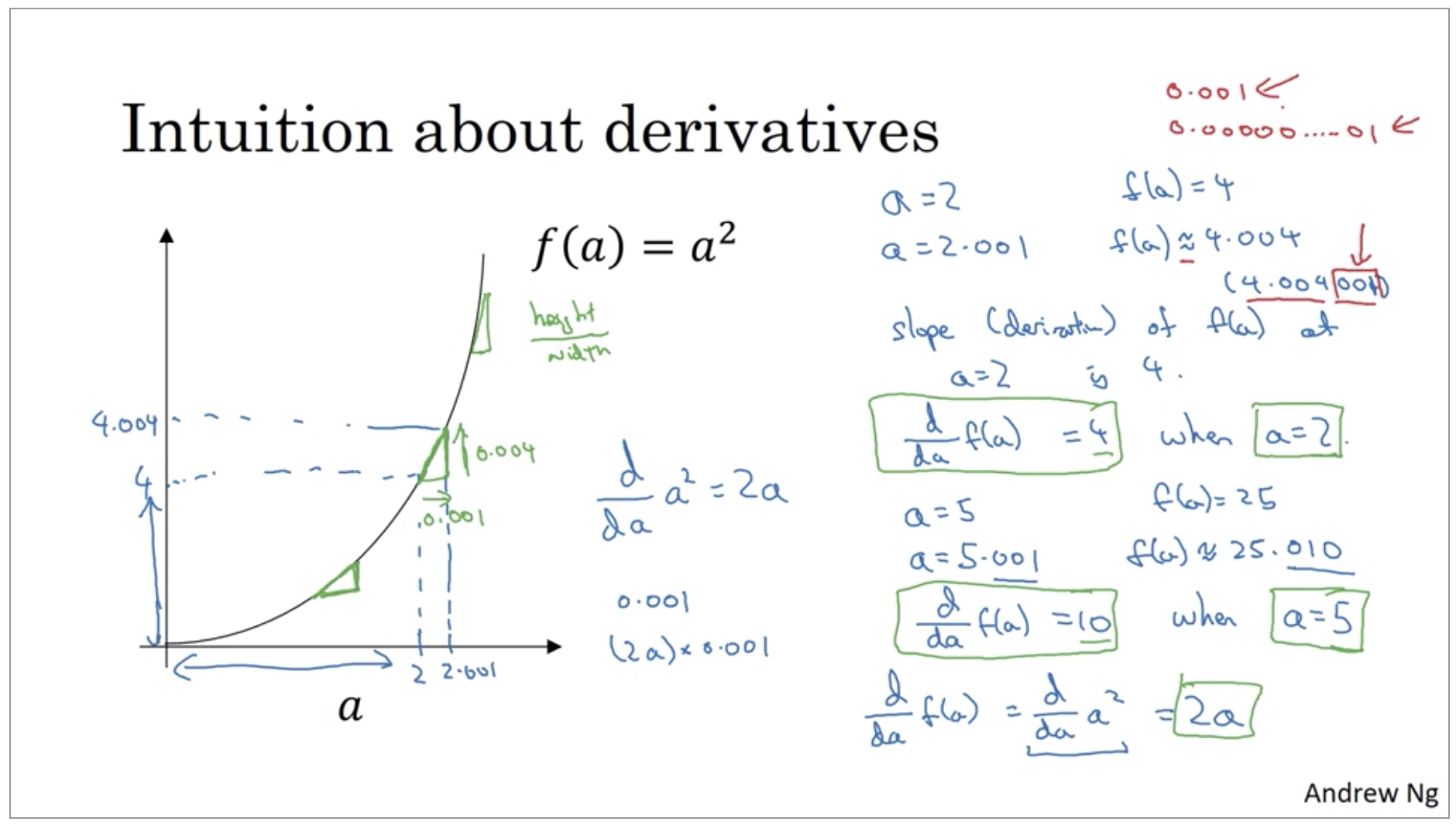
The table formulas and they’ll tell you that derivative of 2 of a^2 is 2a. Namely, when a=2, the slope of function to a is 2\times2=4. And when a=5 then the slope of the function 2a is 2\times5=10.
Now one tiny little detail, I use these approximate symbols here and this wasn’t exactly 4.004, there’s an extra .001 hanging out there. And the reason why is not 4.004 exactly is because derivatives are defined using this infinitesimally small nudges to a rather than 0.001 which is not.
There are just two take messages.
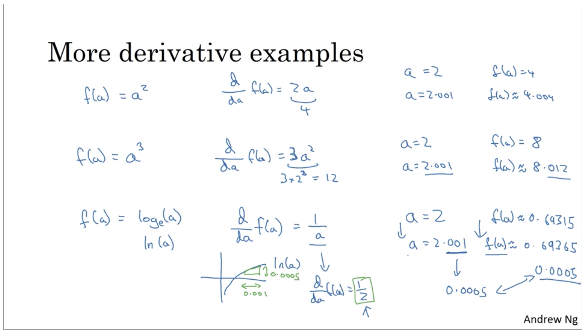
- First is that the derivative of the function just means the slope of a function and the slope of a function can be different at different points on the function. In our first example where f(a) = 3a those a straight line. The derivative was the same everywhere, it was three everywhere. For other functions like f(a) = a^2 or f(a) = log(a), the slope of the line varies. So, the slope or the derivative can be different at different points on the curve. So that’s a first take away. Derivative just means slope of a line.
- Second takeaway is that if you want to look up the derivative of a function, you can flip open your calculus textbook or look up Wikipedia and often get a formula for the slope of these functions at different points. So that, I hope you have an intuitive understanding of derivatives or slopes of lines.
Computation Graph
The computations of a neural network are organized in terms of a forward pass or a forward propagation step, in which we compute the output of the neural network, followed by a backward pass or back propagation step, which we use to compute gradients or compute derivatives. The computation graph explains why it is organized this way.
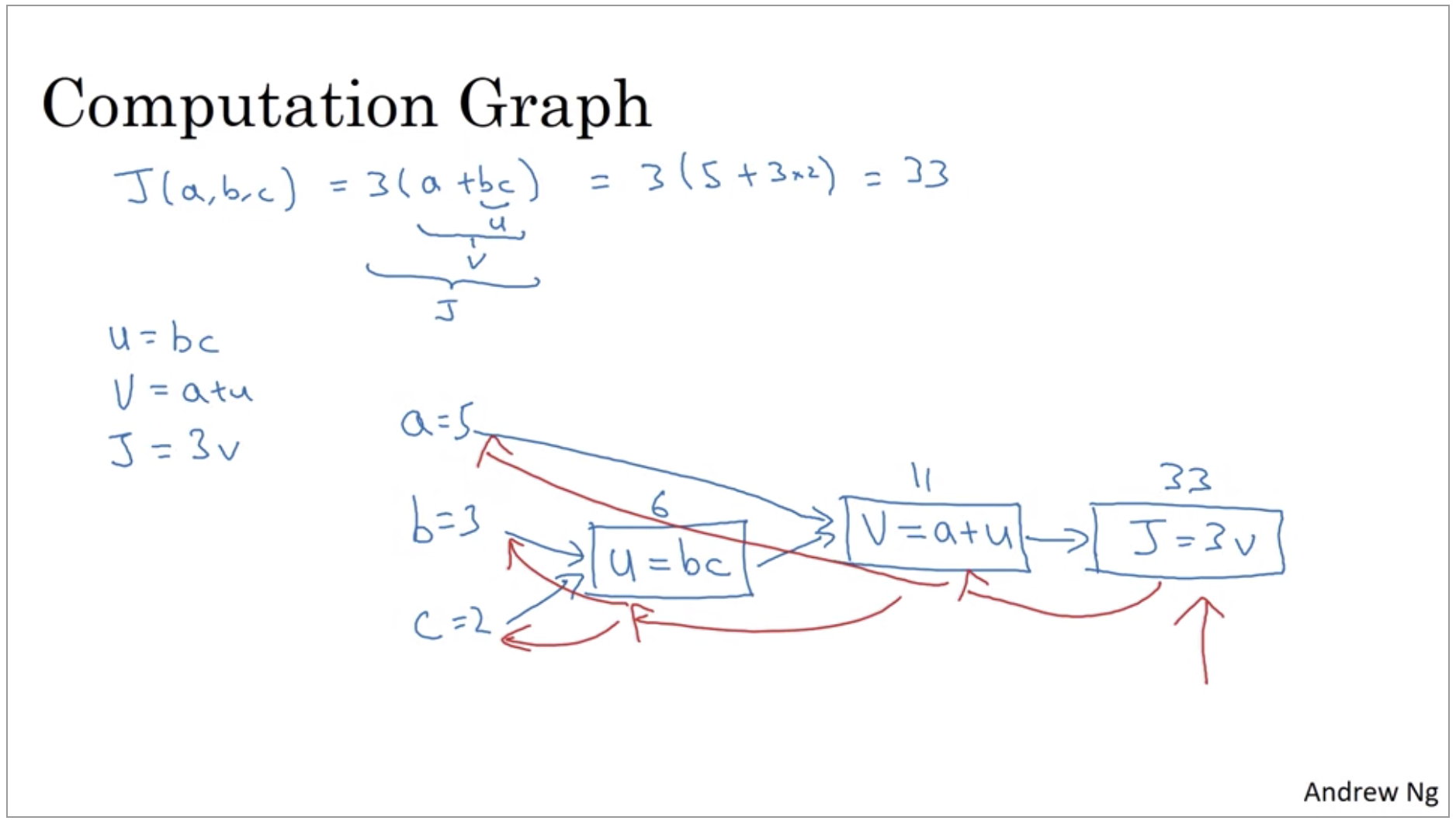
And what we’re seeing in this little example is that, through a left-to-right pass, you can compute the value of J and what we’ll see in order to compute derivatives there’ll be a right-to-left pass like this, kind of going in the opposite direction as the blue arrows. That would be most natural for computing the derivatives.
Derivatives with Computation Graph
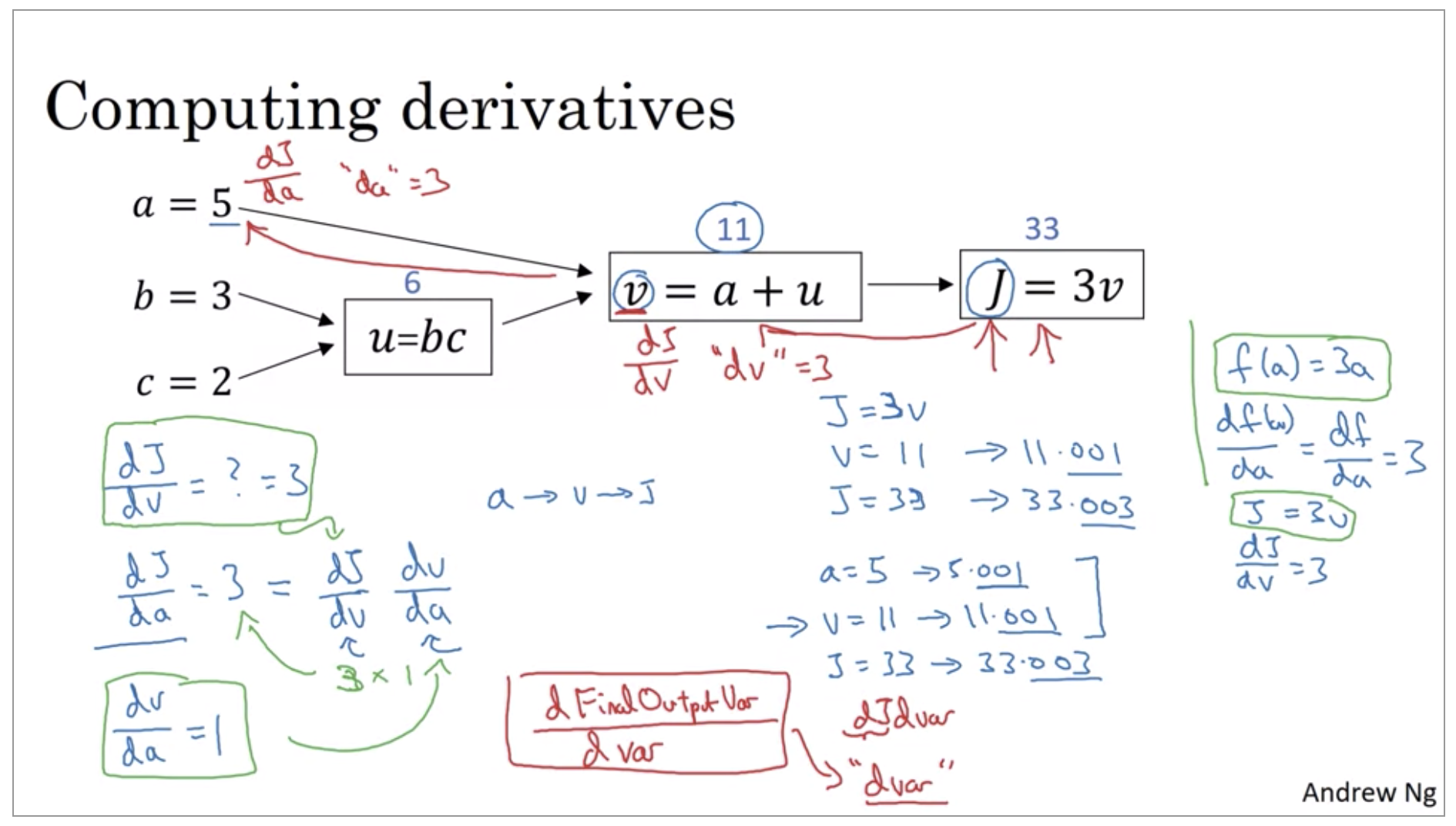
If we’re to bump up v by a little bit to 11.001, then J, which is 3v, so currently 33, will get bumped up to 33.003. So here, we’ve increased v by 0.001. And the net result of that is that J goes out 3 times as much. So the derivative of J with respect to v is equal to 3.
Terminology of back-propagation, what we’re seeing is that if you want to compute the derivative of this final output variable, which usually is a variable you care most about, with respect to v, then we’ve done one step of back-propagation. So we call it one step backwards in this graph.
First, by changing a, you end up increasing v. Well, how much does v increase? It is increased by an amount that’s determined by dv/da. And then the change in v will cause the value of J to also increase. So in calculus, this is actually called the chain rule that if a affects v, affects J, then the amounts that J changes when you nudge a is the product of how much v changes when you nudge a times how much J changes when you nudge v.
So that was the computation graph and how does a forward or left to right calculation to compute the cost function such as J that you might want to optimize. And a backwards or a right to left calculation to compute derivatives.
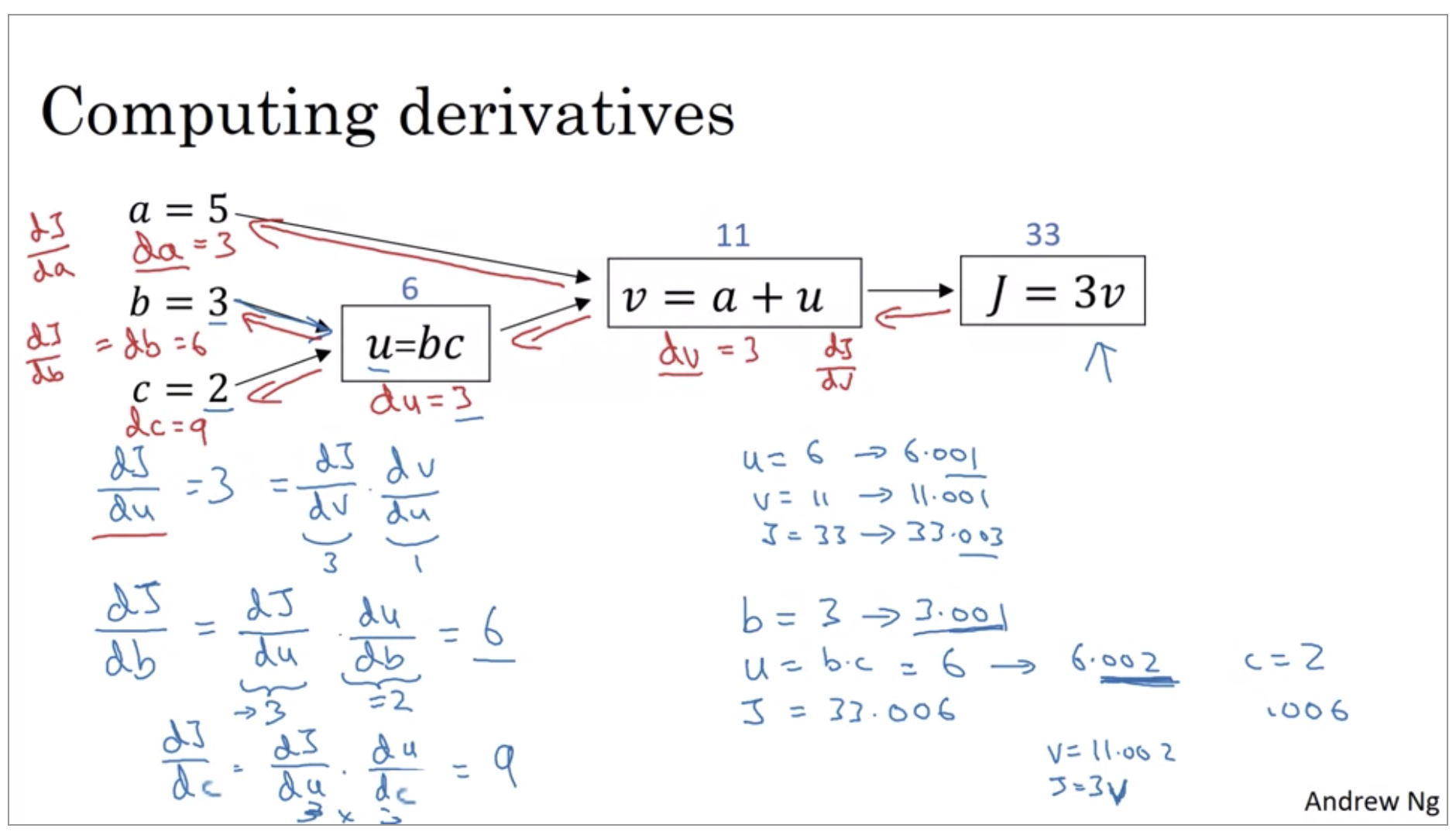
dvar // The derivative of a final output variable with
     // respect to various intermediate quantities.
Logistic Regression Gradient Descent
\[z = w^Tx + b \\ \hat{y}=a=\sigma(z) \\ \mathcal{L}(a,y) = -(ylog(a)+(1-y)log(1-a))\]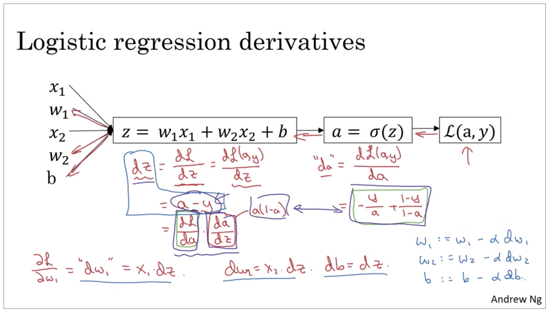
Gradient Descent on m Examples
To get started, let’s remind ourselves of the definition of the cost function J.
\[J(w,b) = \frac{1}{m} \sum_{i=1}^m \mathcal{L} (a^{(i)}, y^{(i)}) \\ a^{(i)} = \hat{y}^{(i)} = \sigma(z^{(i)}) = \sigma(w^Tx^{(i)}+b)\]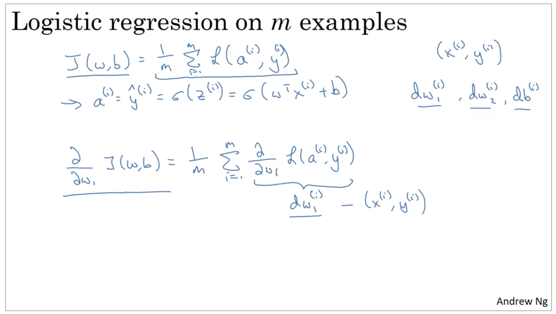
So, now you notice the overall cost functions as a sum was really average, because the one over m term of the individual losses. So, it turns out that the derivative, respect to w_1 of the overall cost function is also going to be the average of derivatives respect to w_1 of the individual lost terms.
But it turns out there are two weaknesses with the calculation as we’ve implemented it here, which is that, to implement logistic regression this way, you need to write two for loops. The first for loop is this for loop over the m training examples, and the second for loop is a for loop over all the features over here.
Python and Vectorization
Vectorization is basically the art of getting rid of explicit for-loop in your code. In the deep learning era, I think the ability to perform vectorization has become a key skill.
Vectorization
\[z=w^Tx + b \\ w \in \R^{n_x}, x \in \R^{n_x}\]import time
a = np.random.rand(1000000)
b = np.random.rand(1000000)
tic = time.time()
c = np.dot(a,b)
toc = time.time()
print(c)
print("Vectorized version:" + str(1000 * (toc - tic)) + "ms")
c = 0
tic = time.time()
for i in range(1000000):
c += a[i] * b[i]
toc = time.time()
print(c)
print("For loop:" + str(1000 * (toc - tic)) + "ms")
250250.50437341325
Vectorized version:1.1546611785888672ms
250250.50437341706
For loop:427.69765853881836ms
The vectorize version took 1.1 milliseconds. The explicit for loop and non-vectorize version took about 400 milliseconds. The non-vectorize version took something like 300 times longer than the vectorize version.
But all the demos I did just now in the Jupiter notebook where actually on the CPU. And it turns out that both GPU and CPU have parallelization instructions. They’re sometimes called SIMD instructions. It’s just that GPUs are remarkably good at these SIMD calculations but CPU is actually also not too bad at that. The rule of thumb to remember is whenever possible, avoid using explicit four loops.
More Vectorization Examples
Whenever possible, avoid explicit for-loops.
# For loop
u = np.zeros((n, 1))
for i in range(n):
  for j in range(m):
    u[i] += A[i][j] * v[:]

# Vectorization
u = np.dot(A, v)
Say you need to apply the exponential operation on every element of a matrix/vector.
# For loop
u = np.zeros((n, 1))
for i in range(n):
  u[i] = math.exp(v[i])

# Vectorization
u = np.exp(v)

# Other Vectorizations
np.log(v)
np.abs(v)
np.maximum(v, 0)
v ** 2
1 / v
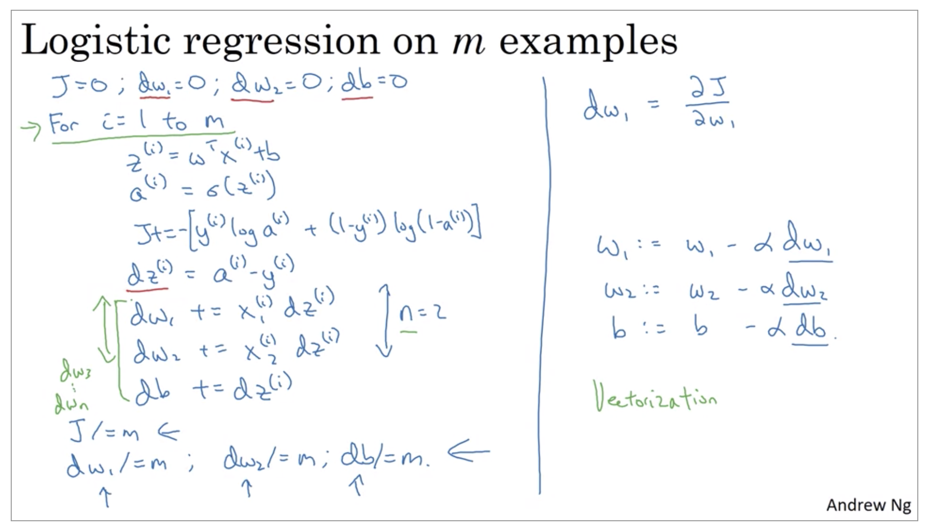
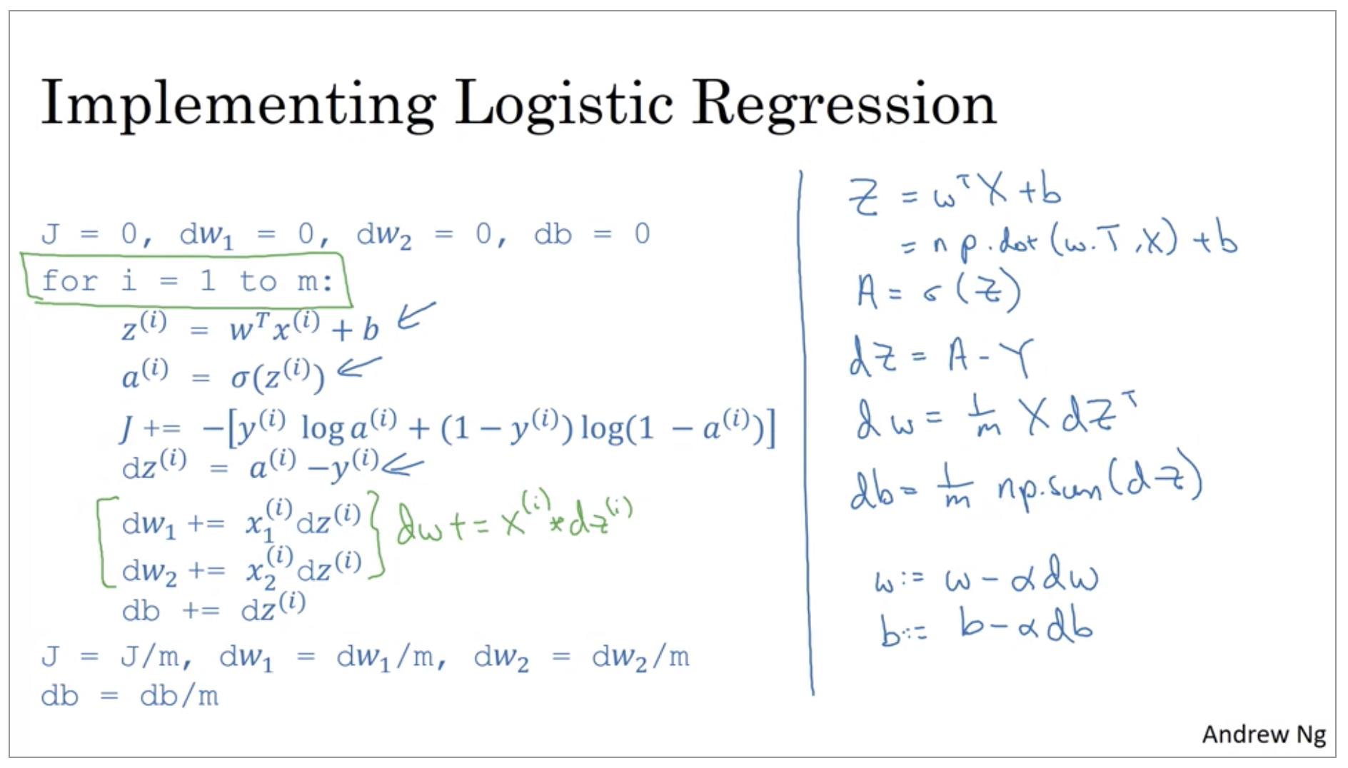
So, let’s take all of these learnings and apply it to our logistic regression gradient descent implementation.
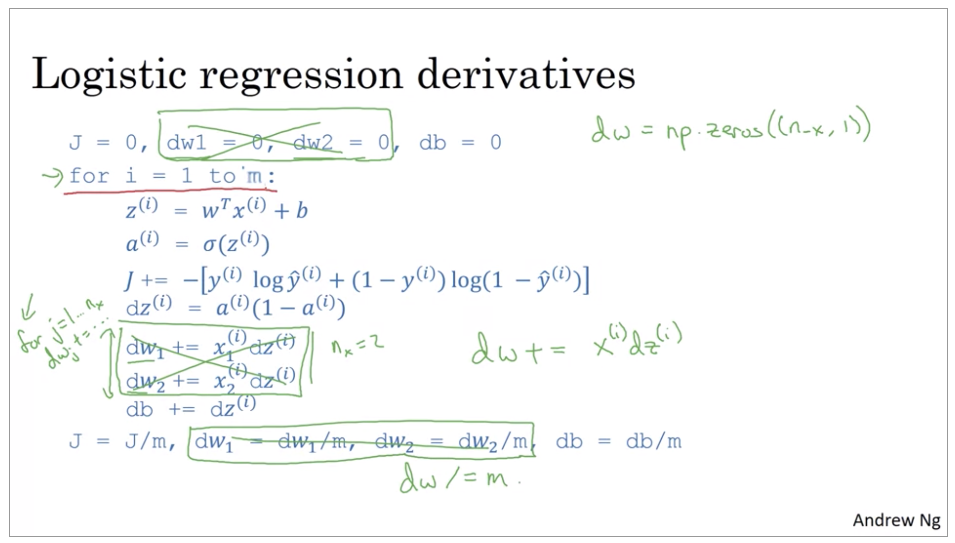
So now we’ve gone from having two for-loops to just one for-loop. We still have this one for-loop that loops over the individual training examples.
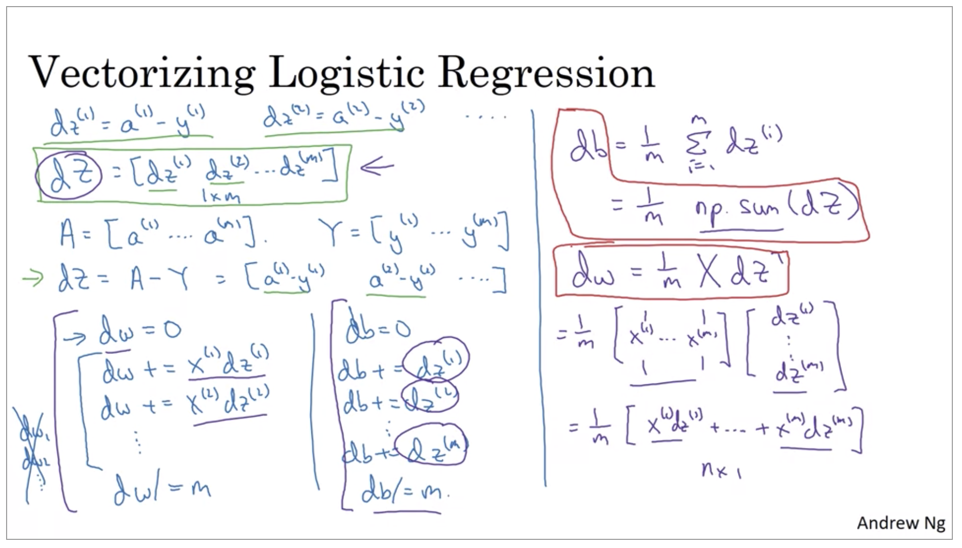
Vectorizing Logistic Regression
You can use vectorization to compute their predictions. You might need to do this M times, if you have M training examples. So, it turns out, that in order to carry out the four propagation step, that is to compute these predictions on our M training examples, there is a way to do so, without needing an explicit for-loop.
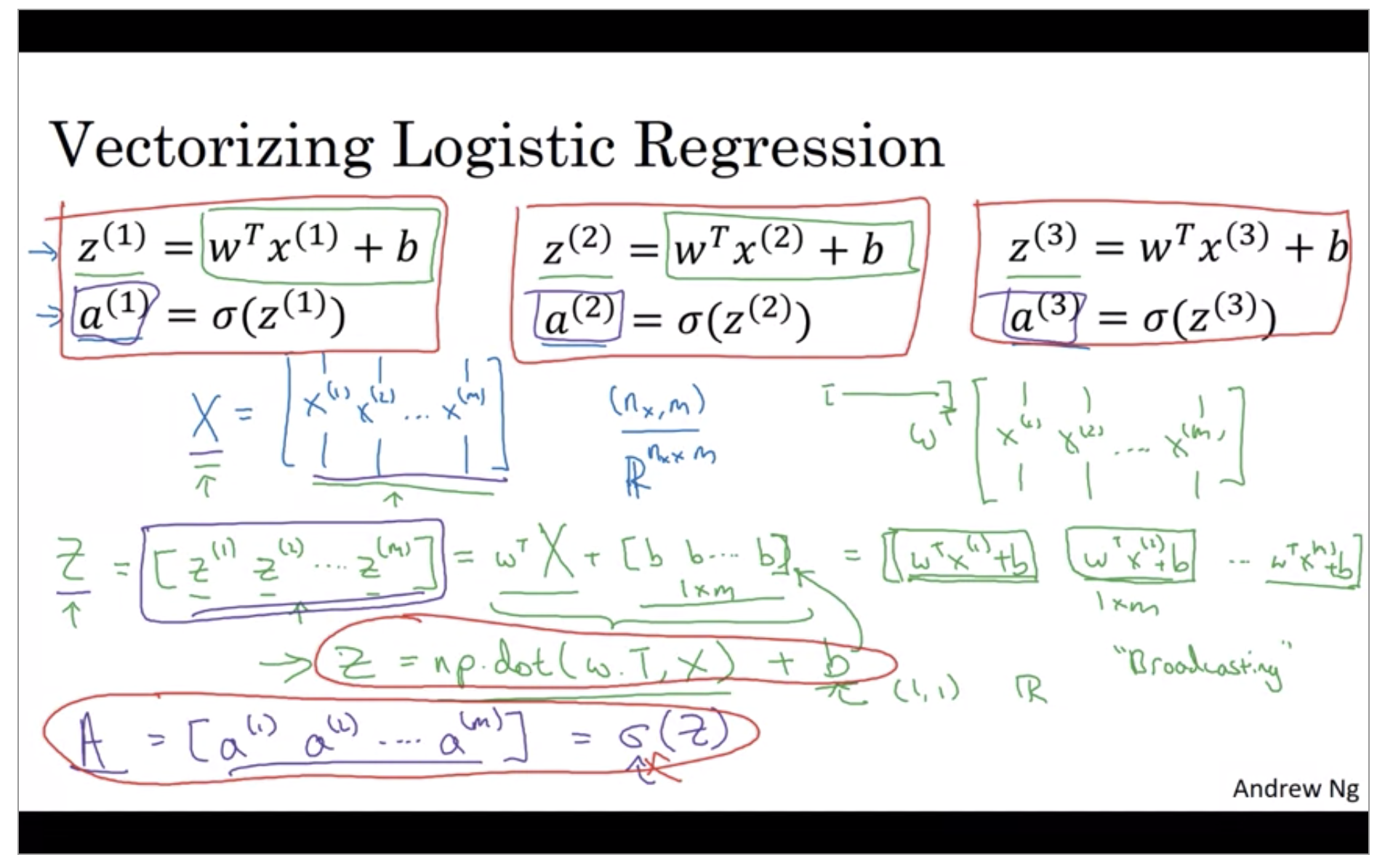
Z = np.dot(w.T, X) + b # python Broadcasting
A = sigmoid(Z)
Vectorizing Logistic Regression’s Gradient Output
We’ll put it all together and show how you can derive a very efficient implementation of logistic regression.
You have just implemented a single iteration of gradient descent for logistic regression.
Now, I know I said that we should get rid of explicit full loops whenever you can but if you want to implement multiple iterations as a gradient descent then you still need a full loop over the number of iterations. So, if you want to have a thousand iterations of gradient descent, you might still need a full loop over the iteration number. There is an outermost full loop like that then I don’t think there is any way to get rid of that for-loop.
Broadcasting in Python
import numpy as np

A = np.array([[56.0, 0.0, 4.4, 68.0],
              [1.2,104.0,52.0,8.0],
              [1.8,135.0,99.0,0.9],
             ])

cal = A.sum(axis=0) # 1 by 4
percentage = 100 * A / (cal) # A(3, 4) / cal(1, 4): broadcasting
A note on python/numpy vectors
import numpy as np
a = np.random.randn(5,) # Don't use rank 1 array
a.reshape((5,1)) # Reshape
print(a.shape)

a = np.random.randn(5,1) # column vector
print(a.shape)

a = np.random.randn(1,5) # row vector
print(a.shape)
And so takeaways are to simplify your code, don’t use rank 1 arrays. Always use either n by one matrices, basically column vectors, or one by n matrices, or basically row vectors.
Logistic regression cost function