DLS Course 1 - Week 3
Shallow Neural Network
Neural Networks Overview
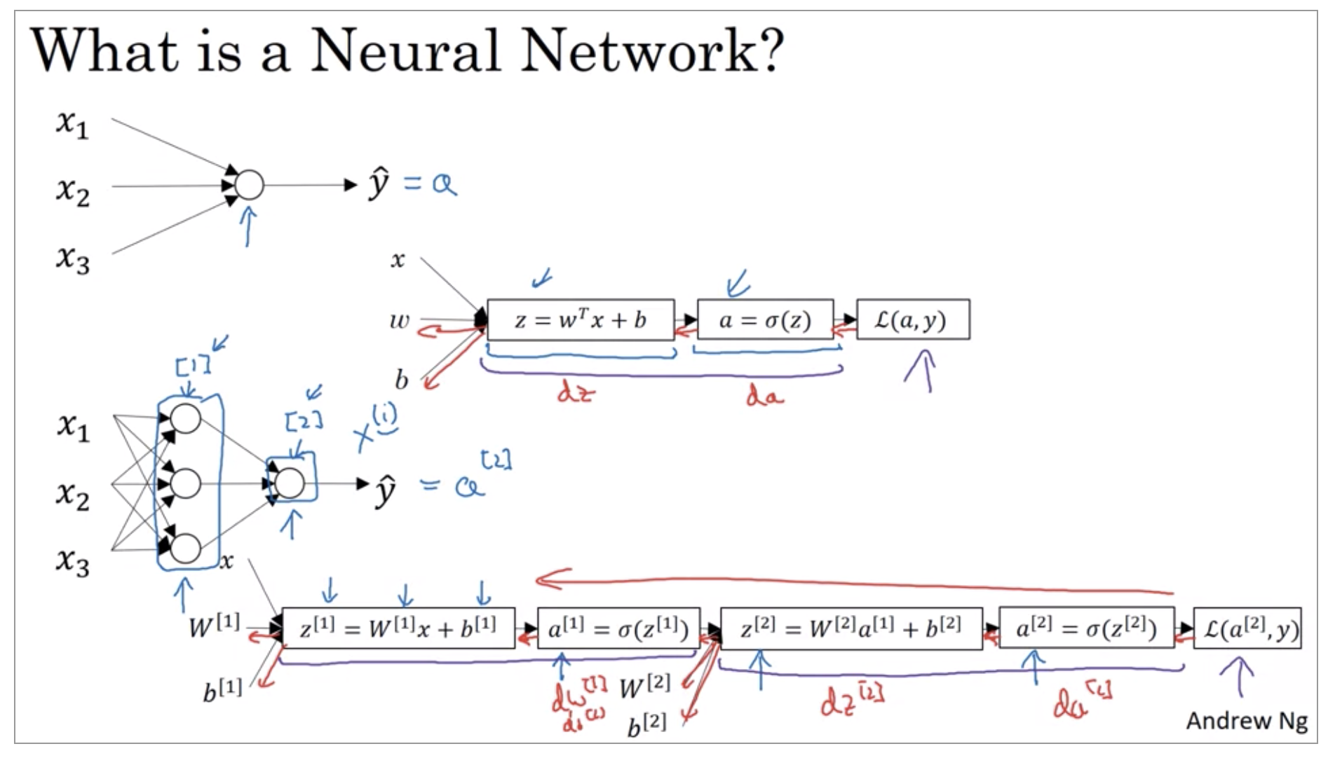
Last week, we had talked about logistic regression, and we saw how this model corresponds to the following computation draft, where you didn’t put the features x and parameters w and b that allows you to compute z which is then used to computes a, and we were using a interchangeably with this output y hat and then you can compute the loss function, L.
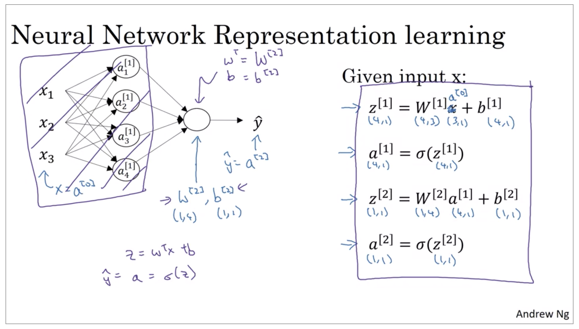
So, new notation that we’ll introduce is that we’ll use superscript square bracket one to refer to quantities associated with this stack of nodes, it’s called a layer.
Neural Network Representation
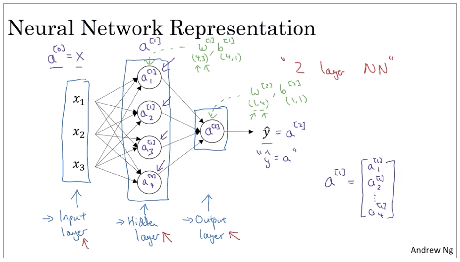
The hidden layer refers to the fact that in the training set, the true values for these nodes in the middle are not observed. That is, you don’t see what they should be in the training set.
The input layer passes on the value x to the hidden layer, so we’re going to call that activations of the input layer A super script 0.
One funny thing about notational conventions in neural networks is that this network that you’ve seen here is called a two layer neural network. And the reason is that when we count layers in neural networks, we don’t count the input layer. So the hidden layer is layer one and the output layer is layer two.
Computing a Neural Network’s Output
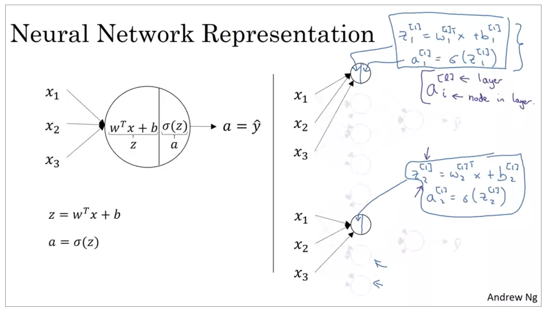
The nodes in the hidden layer does two steps of computation. The first step, it computes z equals w transpose x plus b, and the notation we’ll use is, these are all quantities associated with the first hidden layer. Then second step, is it computes a^{[1]}_1 equals sigmoid of z^{[1]}_1.
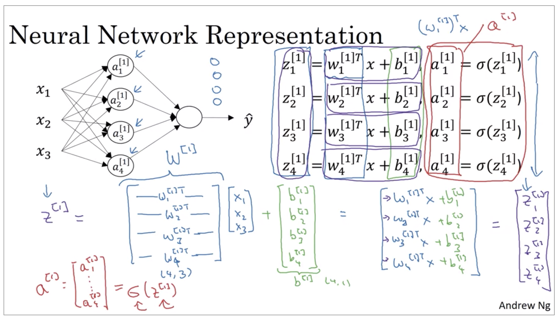
If you’re actually implementing a neural network, doing this with a for loop, seems really inefficient. So, what we’re going to do, is take these four equations and vectorize.
Vectorizing across multiple examples
You saw how to compute the prediction on a neural network, given a single training example. You’ll see how to vectorize across multiple training examples.
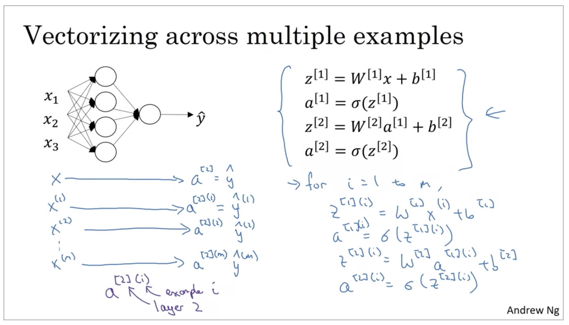
So let me just copy whole block of code to the next slide and then we’ll see how to vectorize this. If you want the analogy is that we went from lower case vector xs to just capital case X matrix by stacking up the lower case xs in different columns.
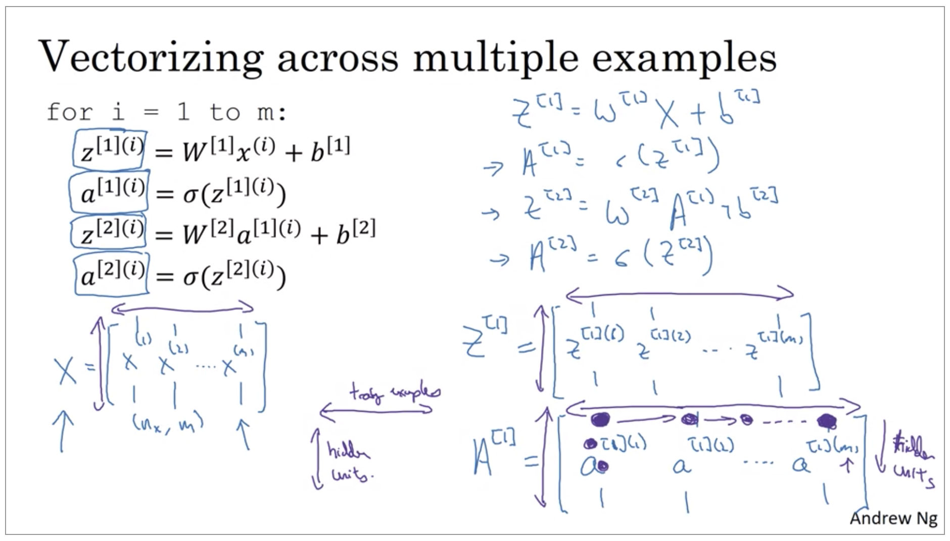
So of these equations, you now know how to implement in your network with vectorization, that is vectorization across multiple examples.
Explanation for Vectorized Implementation
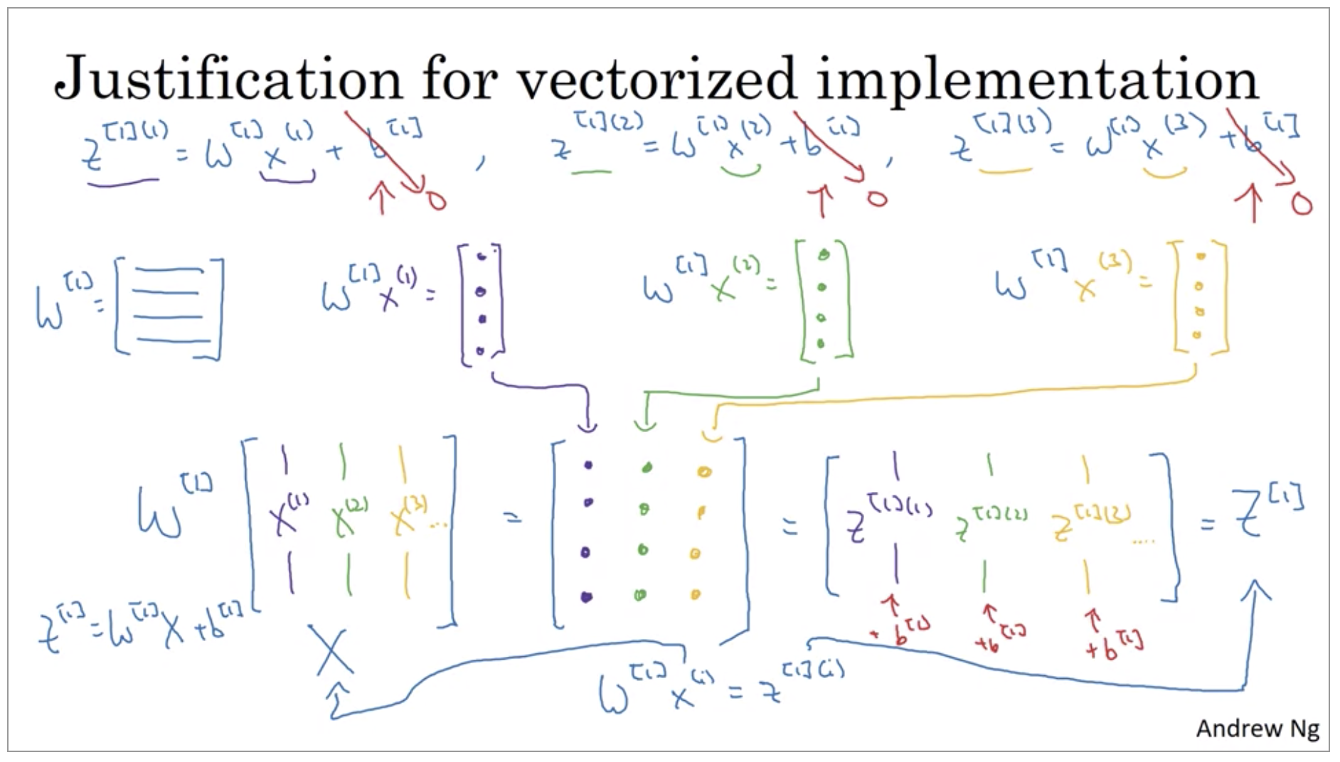
It turns out that a similar analysis allows you to show that the other steps also work on using a very similar logic where if you stack the inputs in columns then after the equation, you get the corresponding outputs also stacked up in columns.
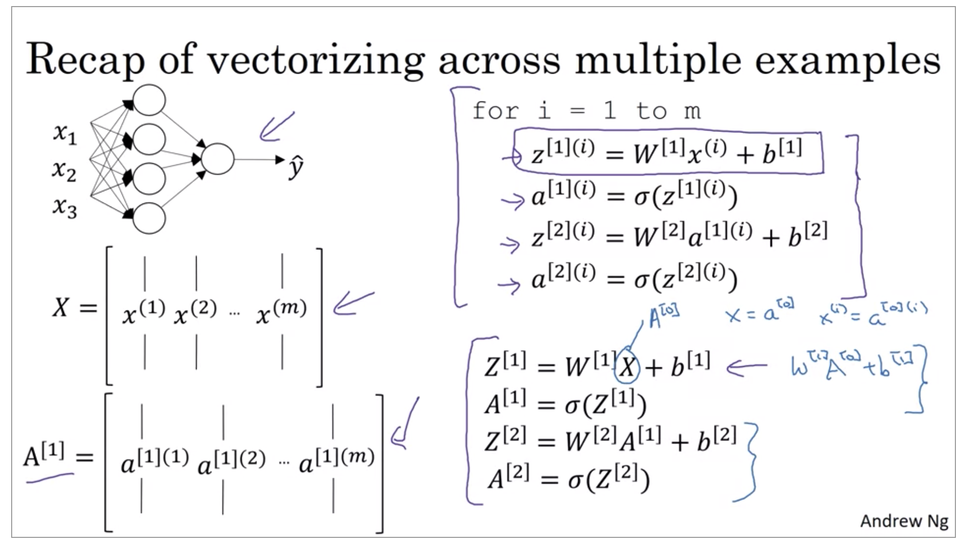
Here we have two-layer neural network.
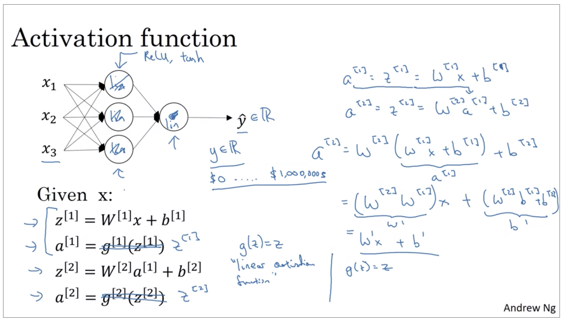
Activation Functions
When you build your neural network, one of the choices you get to make is what activation function to use in the hidden layers, as well as what is the output units of your neural network. So far, we’ve just been using the sigmoid activation function. But sometimes other choices can work much better.
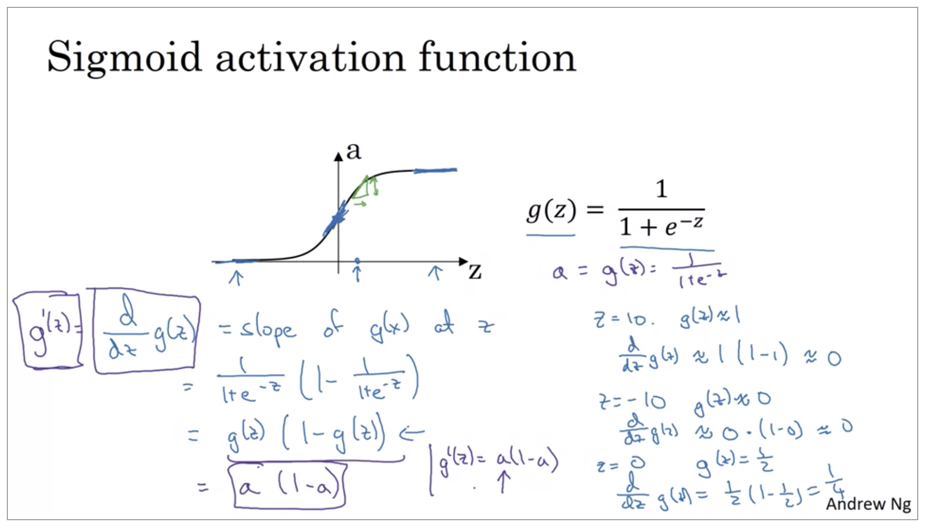
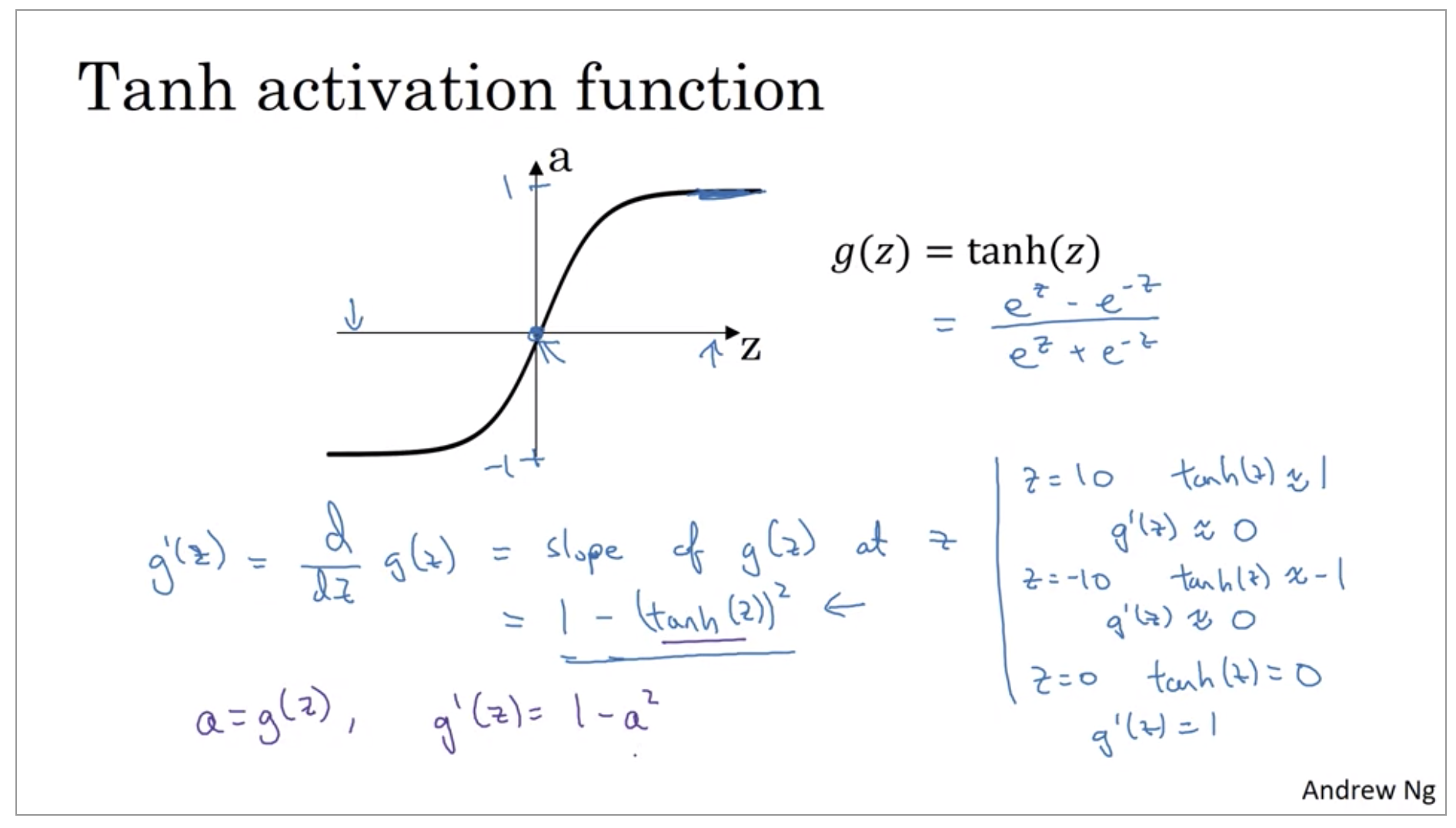
Sigmoid function, Hyperbolic tangent function
So for example, the sigmoid function goes within zero and one, and activation function that almost always works better than the sigmoid function is the tangent function or the hyperbolic tangent function. And it is actually mathematically, a shifted version of the sigmoid function. And it turns out for hidden units, if you let the function g of z be equal to tanh(z), this almost always works better than the sigmoid function because the values between plus 1 and minus 1, the mean of the activations that come out of your hidden layer, and they are closer to having a 0 mean. And so just as sometimes when you train a learning algorithm, you might center the data and have your data have 0 mean using a tanh instead of a sigmoid function. It kind of has the effect of centering your data so that the mean of your data is closer to 0 rather than, maybe 0.5. And this actually makes learning for the next layer a little bit easier.
But one takeaway is that I pretty much never use the sigmoid activation function anymore. The tanh function is almost always strictly superior. The one exception is for the output layer because if y is either 0 or 1, then it makes sense for y hat to be a number, the one to output that’s between 0 and 1 rather than between minus 1 and 1. So the one exception where I would use the sigmoid activation function is when you are using binary classification.
Now, one of the downsides of both the sigmoid function and the tanh function is that if z is either very large or very small, then the gradient or the derivative or the slope of this function becomes very small. So if z is very large or z is very small, the slope of the function ends up being close to 0. And so this can slow down gradient descent.
Here are some rules of thumb for choosing activation functions. If your output is 0, 1 value, if you’re using binary classification, then the sigmoid activation function is a very natural choice for the output layer.
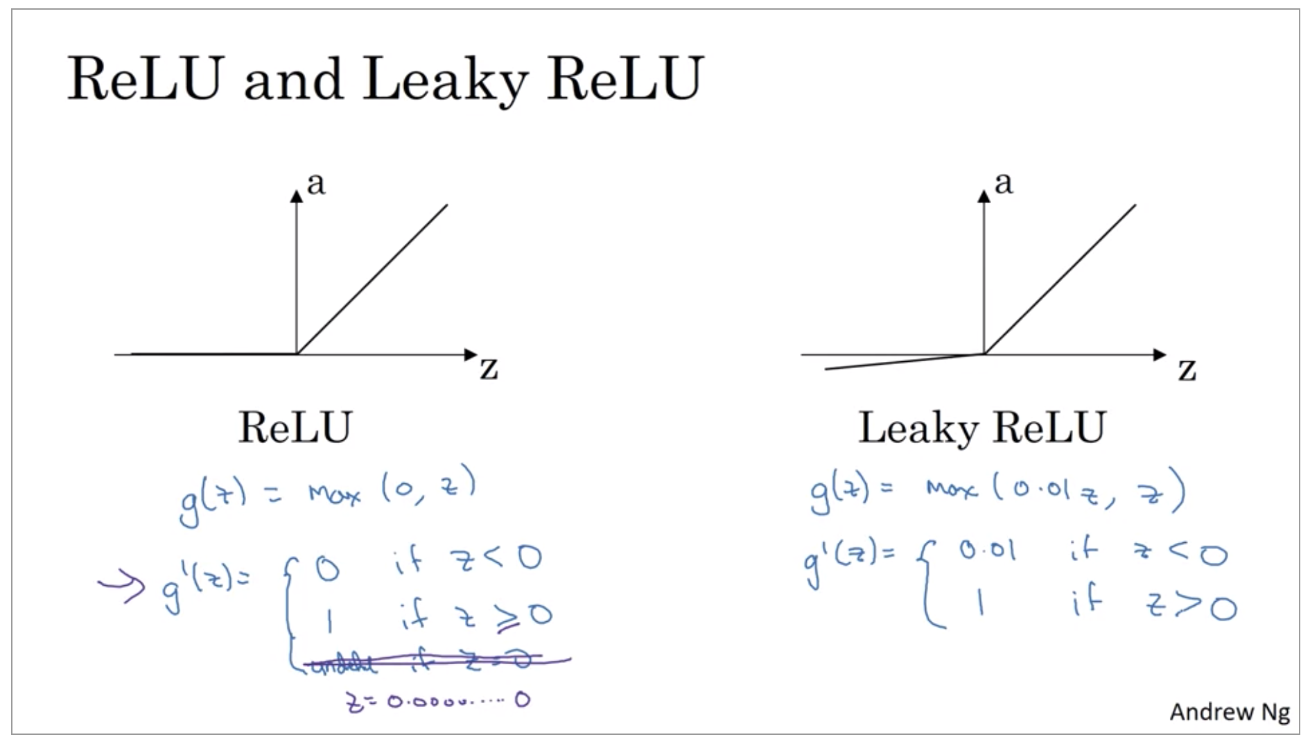
ReLU, leaky ReLU
For all other unit’s ReLU, or the rectified linear unit is increasingly the default choice of activation function. One disadvantage of the ReLU is that the derivative is equal to zero, when z is negative. In practice, this works just fine. There is a another version of ReLU takes a slight slope like so, so this is called the leaky ReLU. This usually works better than the ReLU activation function, although it’s just not used as much in practice. Either one should be fine, although, if you had to pick one, I usually just use the ReLU.
And the advantage of both the ReLU and the leaky ReLU is that for a lot of the space of Z, the derivative of the activation function, the slope of the activation function is very different from 0. And so in practice, using the ReLU activation function, your neural network will often learn much faster than when using the tanh or the sigmoid activation function.
But if you feel like trying that in your application, please feel free to do so. And you can just see how it works, and how well it works, and stick with it if it gives you a good result.
One of the themes we’ll see in deep learning is that you often have a lot of different choices in how you code your neural network. Ranging from number of hidden units, to the choice activation function, to how you initialize the ways which we’ll see later. A lot of choices like that. And it turns out that it’s sometimes difficult to get good guidelines for exactly what would work best for your problem.
So a common piece of advice would be, if you’re not sure which one of these activation functions work best, try them all, and evaluate on a holdout validation set, or a development set, which we’ll talk about later, and see which one works better, and then go with that.
Why do you need non-linear activation functions?
If you were to use linear activation functions or we can also call them identity activation functions, then the neural network is just outputting a linear function of the input. And we’ll talk about deep networks later, neural networks with many, many layers, many hidden layers. And it turns out that if you use a linear activation function or alternatively, if you don’t have an activation function, then no matter how many layers your neural network has, all it’s doing is just computing a linear activation function.
There is just one place where you might use a linear activation function. g(x) = z. that’s if you are doing machine learning on the regression problem. So if y is a real number. So for example, if you’re trying to predict housing prices. So y is not 0, 1, but is a real number.
Derivatives of activation functions
For the value g of z is equal to max of 0,z, so the derivative is equal to, turns out to be 0 , if z is less than 0 and 1 if z is greater than 0. It’s actually undefined if z is equal to exactly 0. But if you’re implementing this in software, it might not be a 100 percent mathematically correct, but it’ll work just fine if z is exactly a 0, if you set the derivative to be equal to 1.
Gradient descent for Neural Networks
Features:
\[n_x = n^{[0]}, n^{[1]}, n^{[2]} = 1\]Parameters:
\[w^{[1]}, b^{[1]}, w^{[2]}, b^{[2]}\]Cost function:
\[J(w^{[1]}, b^{[1]}, w^{[2]}, b^{[2]}) = \frac{1}{m} \sum_{i=1}^n \mathcal{L}(\hat{y},y) \\ \hat{y} =a^{[2]}\]Gradient descent: repeat {
\[\text{Compute predicts } (\hat{y}^{(i)}, i=1,...m)\] \[dw^{[1]} = \frac{\partial J}{\partial w^{[1]}}, db^{[1]} = \frac{\partial J}{\partial b^{[1]}}, ...\] \[w^{[1]} := w^{[1]} - \alpha dw^{[i]}, b^{[1]} := b^{[1]} - \alpha db^{[1]}, ...\]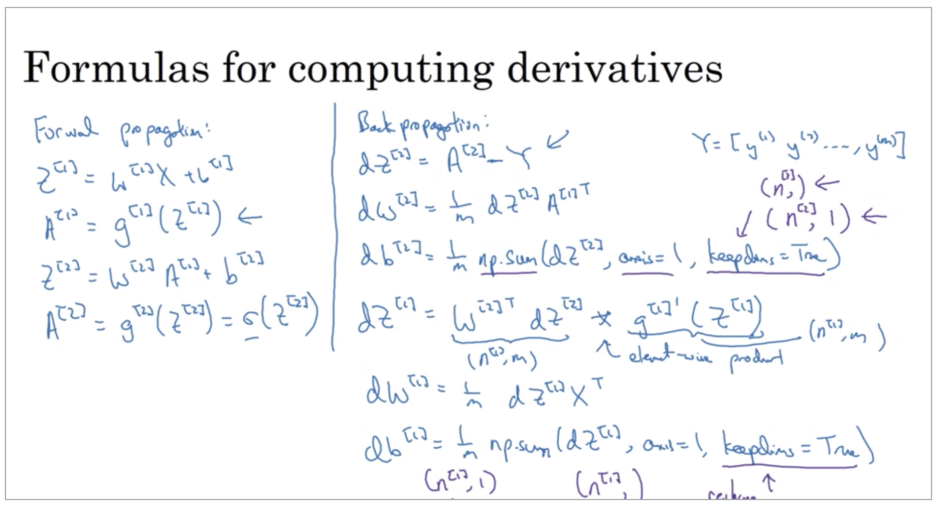
You’ll be able to compute the derivatives you need in order to apply gradient descent, to learn the parameters of your neural network. It is possible to implement this algorithm and get it to work without deeply understanding the calculus. A lot of successful deep learning practitioners do so.
Random Initialization
When you train your neural network, it’s important to initialize the weights randomly. For logistic regression, it was okay to initialize the weights to zero. But for a neural network of initialize the weights to parameters to all zero and then applied gradient descent, it won’t work.

If you initialize the weights to zero, then all of your hidden units are symmetric. And no matter how long you’re upgrading the center, all continue to compute exactly the same function. So that’s not helpful, because you want the different hidden units to compute different functions. The solution to this is to initialize your parameters randomly.
It turns out that b does not have the symmetry problem, what’s called the symmetry breaking problem. So it’s okay to initialize b to just zeros.
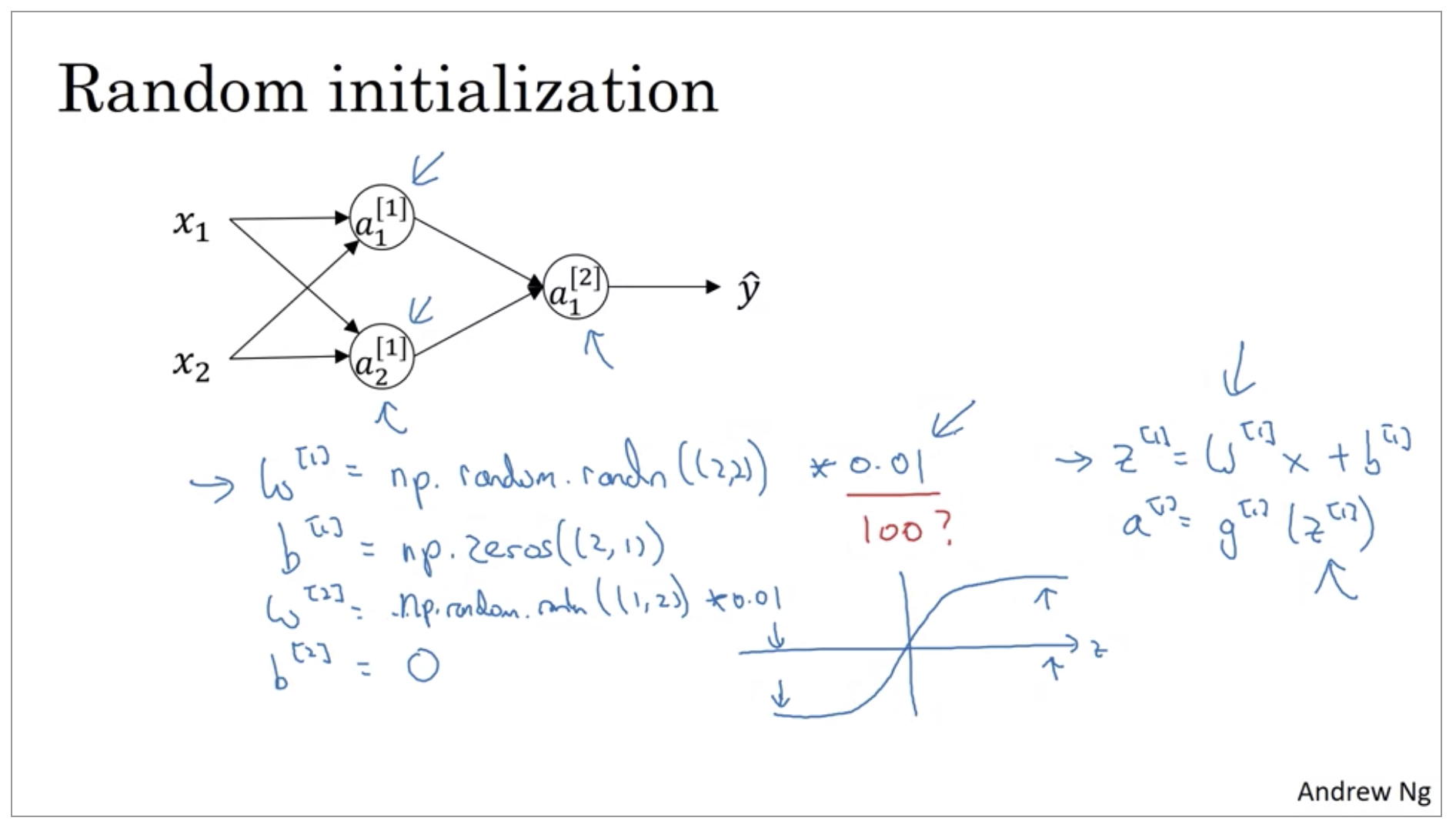
So you might be wondering, where did this constant come from and why is it 0.01? Why not put the number 100 or 1000? Turns out that we usually prefer to initialize the weights to very small random values. Because if you are using a tanh or sigmoid activation function, or the other sigmoid, even just at the output layer. If the weights are too large, then when you compute the activation values, remember that z[1]=w1 x + b. And then a1 is the activation function applied to z1. So if w is very big, z will be very, or at least some values of z will be either very large or very small. And so in that case, you’re more likely to end up at these fat parts of the tanh function or the sigmoid function, where the slope or the gradient is very small. Meaning that gradient descent will be very slow.
finally, it turns out that sometimes they can be better constants than 0.01. When you’re training a neural network with just one hidden layer, it is a relatively shallow neural network, without too many hidden layers. Set it to 0.01 will probably work okay. But when you’re training a very very deep neural network, then you might want to pick a different constant than 0.01.