DLS Course 1 - Week 4
Deep L-layer neural network
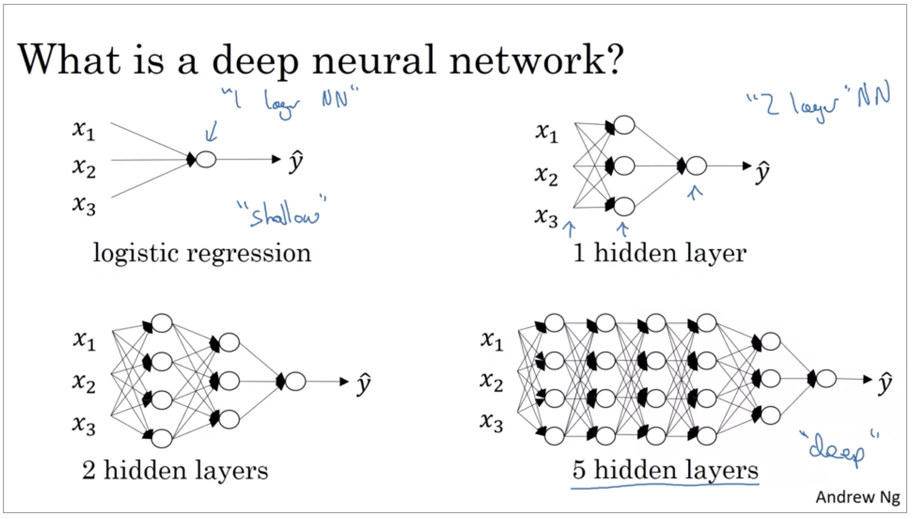
On the machine learning community, has realized that there are functions that very deep neural networks can learn and shallower models are often unable to.
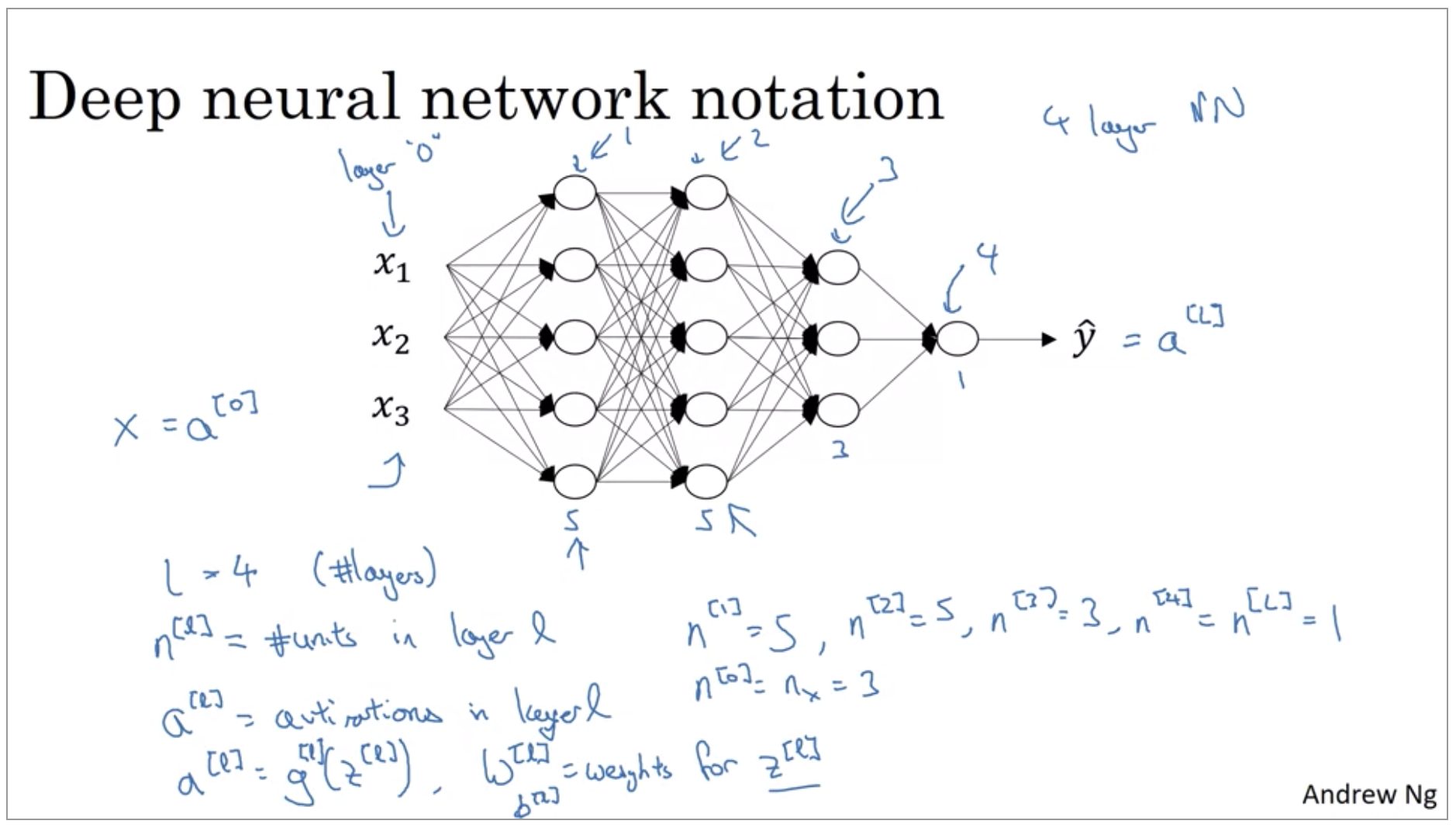
- \(L\) = 4 (number of layers)
- \(n^{[l]}\) = number of units in layer l
- \(a^{[l]}\) = activations in layer l
- \(a^{[l]}\) = \(g^{[l]}(z^{(l)})\), \(w^{[l]}\) = weights for \(z^{[l]}\)
Forward Propagation in a Deep Network
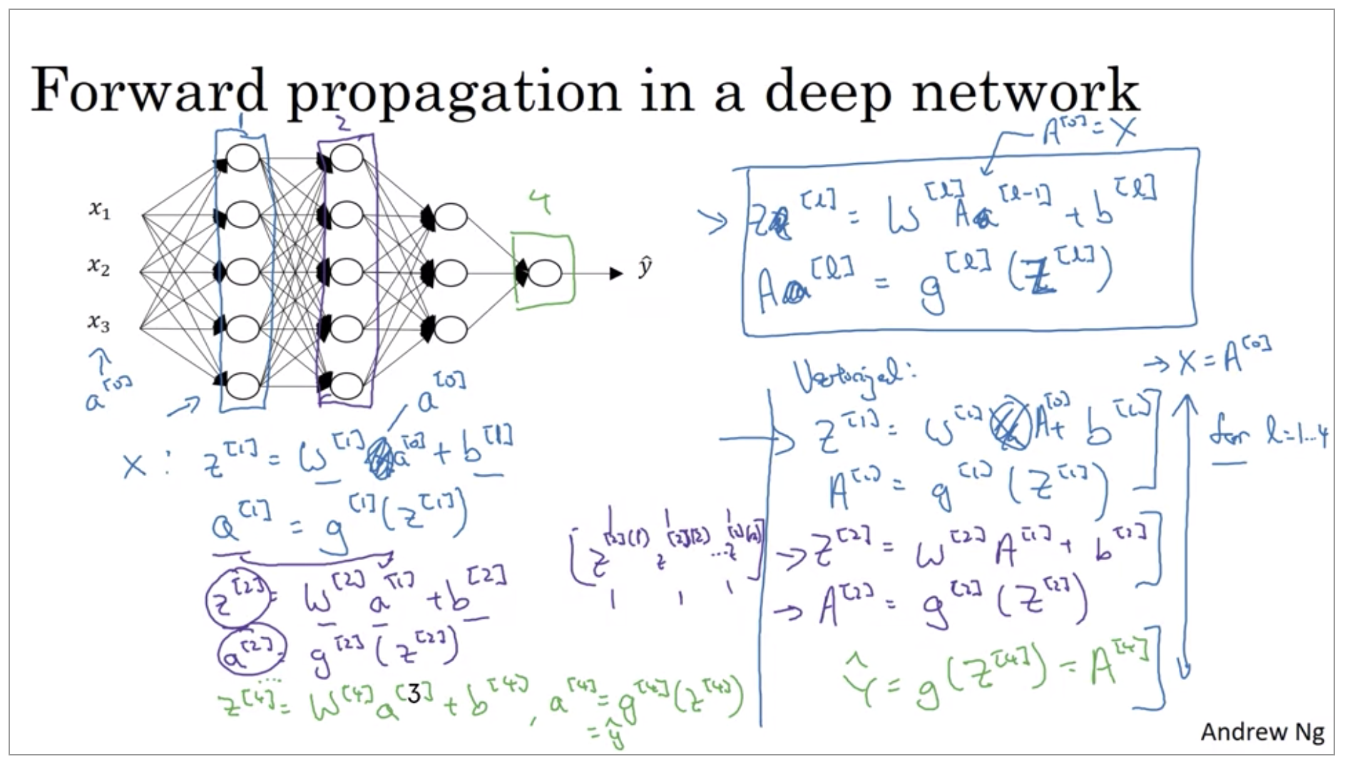
I know that when implementing neural networks, we usually want to get rid of explicit For loops. But this is one place where I don’t think there’s any way to implement this without an explicit For loop. So when implementing forward propagation, it is perfectly okay to have a For loop to compute the activations for layer one, then layer two, then layer three, then layer four.
Getting your matrix dimensions right
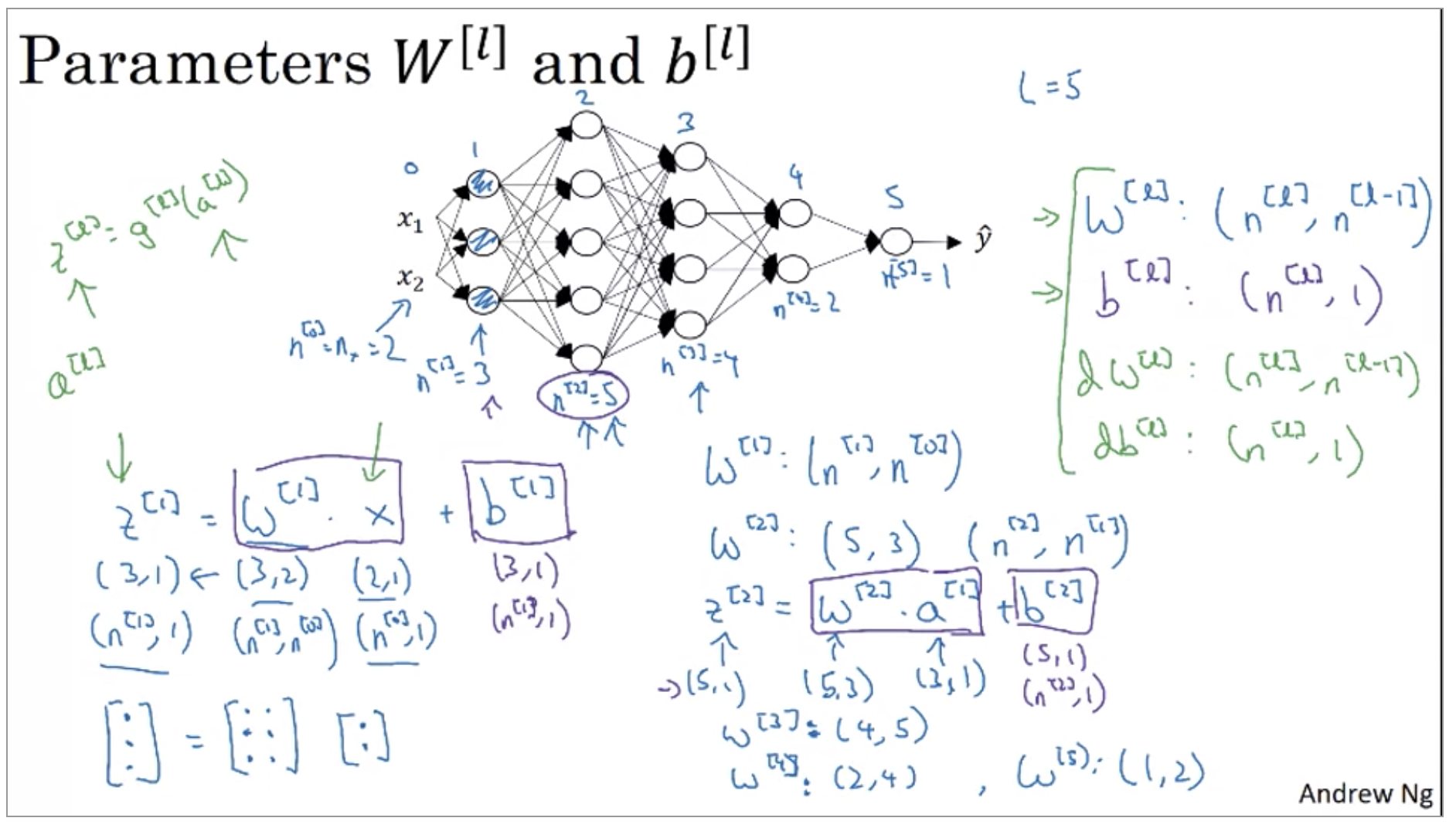
- \(W^{[l]}\): \((n^{[l]}, n^{[l-1]})\)
- \(b^{[l]}\): \((n^{[l]}, 1)\)
- \(dW^{[l]}\): \((n^{[l]}, n^{[l-1]})\)
- \(db^{[l]}\): \((n^{[l]}, 1)\)
Now let’s see what happens when you have a vectorized implementation that looks at multiple examples at a time. Even for a vectorized implementation, of course, the dimensions of wb, dw, and db will stay the same. But the dimensions of z, a, as well as x will change a bit in your vectorized implementation.
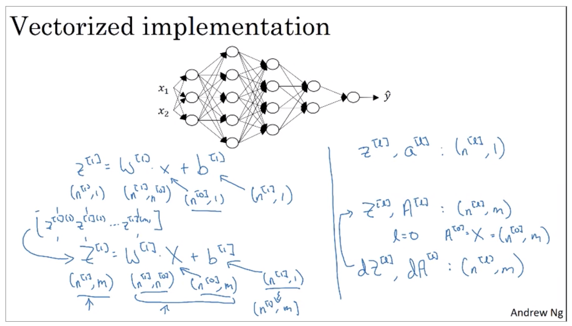
So the dimension of z1 is that, instead of being n1 by 1, it ends up being n1 by m, and m is the size you’re trying to set. The dimensions of w1 stays the same, so it’s still n1 by n0. And x, instead of being n0 by 1 is now all your training examples stacked horizontally. So it’s now n 0 by m, and so you notice that when you take a n1 by n0 matrix and multiply that by an n0 by m matrix. That together they actually give you an n1 by m dimensional matrix, as expected.
Now, the final detail is that b1 is still n1 by 1, but when you take this and add it to b, then through Python broadcasting, this will get duplicated and turn n1 by m matrix, and then add the element wise.
Why deep representations?
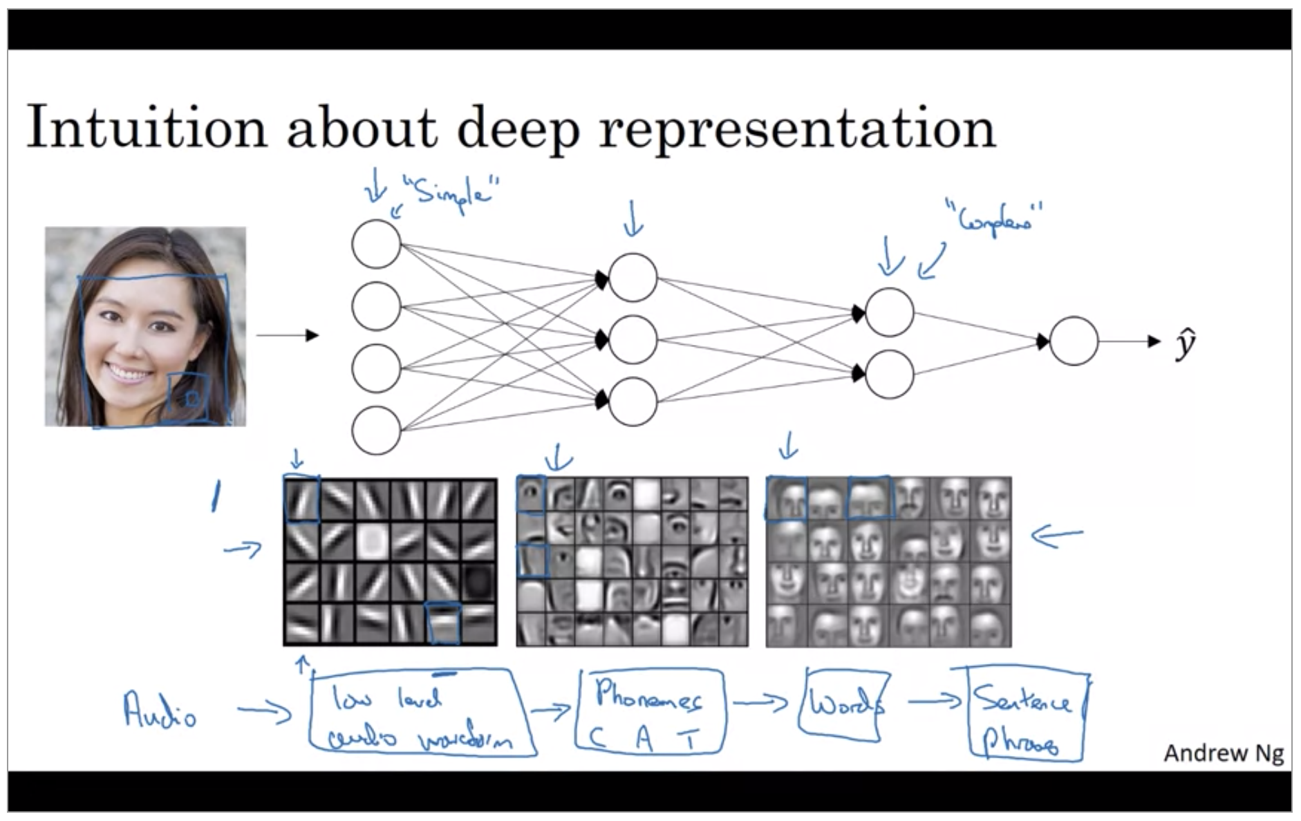
These visualizations will make more sense when we talk about convolutional nets. The main intuition you take away from this is just finding simple things like edges and then building them up. Composing them together to detect more complex things like an eye or a nose then composing those together to find even more complex things. And this type of simple to complex hierarchical representation, or compositional representation, applies in other types of data than images and face recognition as well.
I think analogies between deep learning and the human brain are sometimes a little bit dangerous. But there is a lot of truth to, this being how we think that human brain works and that the human brain probably detects simple things like edges first then put them together to from more and more complex objects and so that has served as a loose form of inspiration for some deep learning as well.
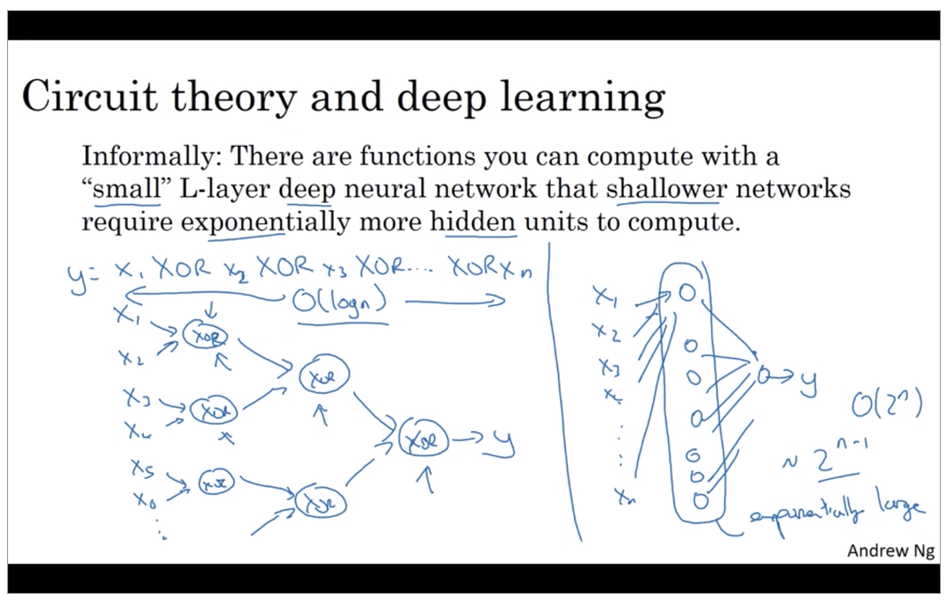
The other piece of intuition about why deep networks seem to work well is the following. So this result comes from circuit theory of which pertains the thinking about what types of functions you can compute with different AND gates, OR gates, NOT gates, basically logic gates.
So to compute XOR, the depth of the network will be on the order of log N. We’ll just have an XOR tree. So the number of nodes or the number of circuit components or the number of gates in this network is not that large. You don’t need that many gates in order to compute the exclusive OR.
if you’re forced to compute this function with just one hidden layer, so you have all these things going into the hidden units. You need to exhaustively enumerate order 2 to the N possible configurations. So you end up needing a hidden layer that is exponentially large in the number of bits.
Now, in addition to this reasons for preferring deep neural networks, to be perfectly honest, I think the other reasons the term deep learning has taken off is just branding. This things just we call neural networks with a lot of hidden layers, but the phrase deep learning is just a great brand, it’s just so deep. Neural networks with many hidden layers rebranded, help to capture the popular imagination as well. But regardless of the PR branding, deep networks do work well. Sometimes people go overboard and insist on using tons of hidden layers. But when I’m starting out a new problem, I’ll often really start out with even logistic regression then try something with one or two hidden layers and use that as a hyper parameter.
Building blocks of deep neural networks
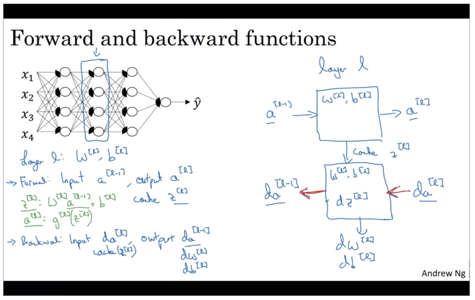
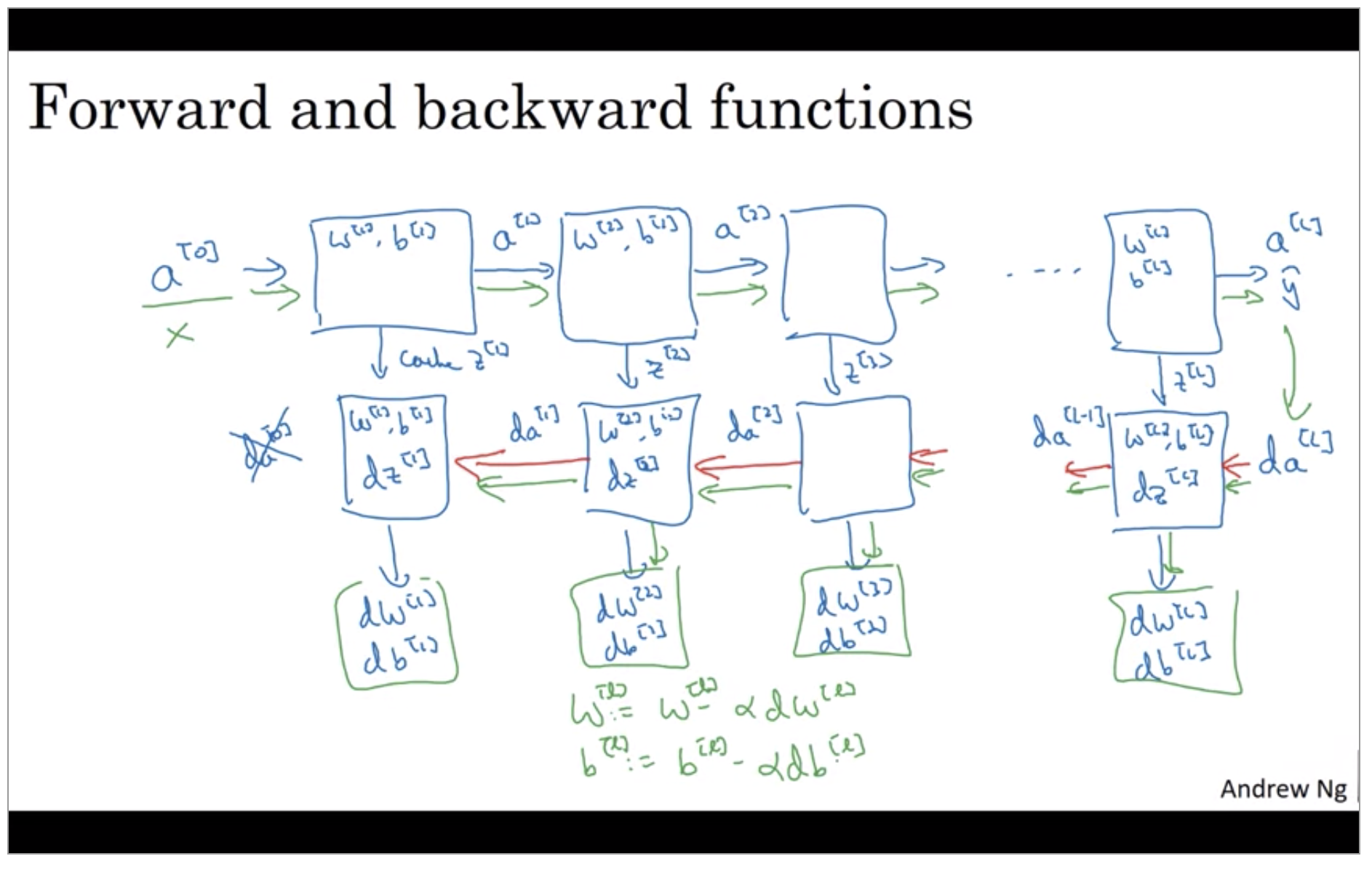
So if you can implement these two functions then the basic computation of the neural network will be as follows.
Forward and Backward Propagation
Forward propagation for layer l
- Input: \(a^{[l-1]}\)
- Output \(a^{[l]}, cache(z^{[l]})\)
-
Single implementation
\[z^{[l]} = W^{[l]}a^{[l-1]} + b^{[l]} \\ a^{[l]} = g^{[l]}(z^{[l]})\] - Vectorize implementation
Backward propagation for layer l
- Input: \(da^{[l]}\)
- Output \(da^{[l-1]}, dW^{[l]}, db^{[l]}\)
-
Single implementation
\[dz^{[l]} = da^{[l]} * g^{[l]'}(z^{[l]}) \\ dW^{[l]} = dz^{[l]} a^{[l-1]} \\ db^{[l]} = dz^{[l]} \\ da^{[l-1]} = W^{[l]T}dz^{[l]} \\ dz^{[l]} = W^{[l+1]T}dz^{[l+1]} * g^{[l]'}(dz^{[l]})\] -
Vectorize implementation
\[dZ^{[l]} = dA^{[l]} * g^{[l]'}(Z^{[l]}) \\ dW^{[l]} = \frac{1}{m}dZ^{[l]} A^{[l-1]T} \\ db^{[l]} = \frac{1}{m} np.sum(dZ^{[l]}, axis=1,keepdim=True) \\ dA^{[l-1]} = W^{[l]T} dZ^{[l]}\]- (* : element-wise product)
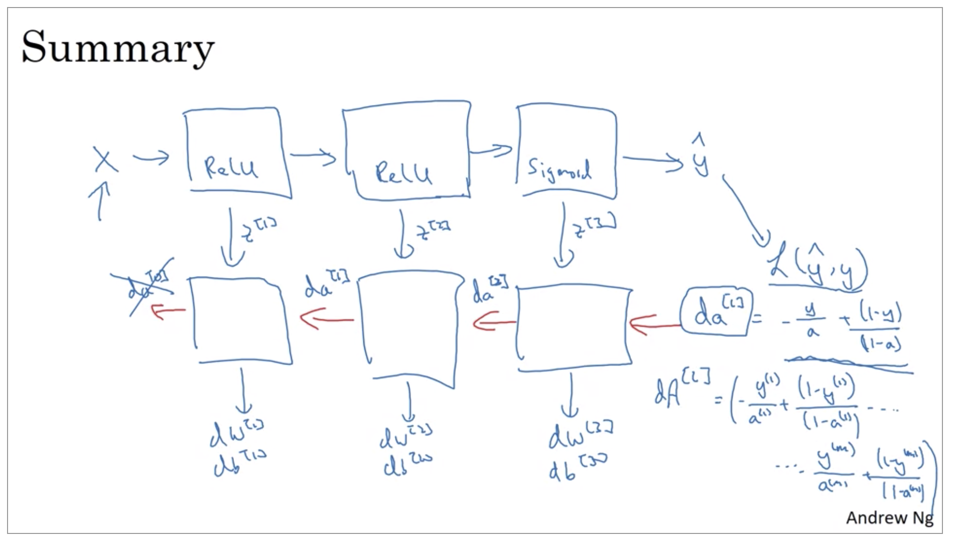
Now, there’s just one last detail that I didn’t talk about which is for the forward recursion, we will initialize it with the input data X. How about the backward recursion? Well, it turns out that \(da[l]\), when you’re using logistic regression, when you’re doing binary classification, is equal to \(\frac{y}{a} + \frac{1-y}{1-a}\). So it turns out that the derivative for the loss function, respect to the output, with respect to \(\hat{y}\), can be shown to be what it is.
-
Single implementation
\[da^{[L]} = -\frac{y}{a} + \frac{(1-y)}{(1-a)}\] -
Vectorize implementation
\[dA^{[L]} = -\frac{y^{(1)}}{a^{(1)}} + \frac{(1-y^{(1)})}{(1-a^{(1)})} + ... -\frac{y^{(m)}}{a^{(m)}} + \frac{(1-y^{(m)})}{(1-a^{(m)})}\]
Although I have to say, even today, when I implement a learning algorithm, sometimes, even I’m surprised when my learning algorithms implementation works and it’s because a lot of complexity of machine learning comes from the data rather than from the lines of code. So sometimes, you feel like, you implement a few lines of code, not quite sure what it did, but this almost magically works, because a lot of magic is actually not in the piece of code you write, which is often not too long. It’s not exactly simple, but it’s not ten thousand, a hundred thousand lines of code, but your feeding so much data that sometimes, even though I’ve worked in machine learning for a long time, sometimes, it still surprises me a bit when my learning algorithm works because a lot of complexity of your learning algorithm comes from the data rather than necessarily from your writing thousands and thousands of lines of code.
Parameters vs Hyper-parameters
- Parameters: \(W^{[1]}, b^{[1]}, W^{[2]}, b^{[2]}, ...\)
- Hyper-parameters
- Learning rate: \(\alpha\)
- #iterations
- #hidden layers: \(L\)
- #hidden units: \(n^{[1]}, n^{[2]}, ...\)
- choice of activation function
- More Hyper-parameters
- various forms of regularization parameters
- mini-batch size
- Momentom
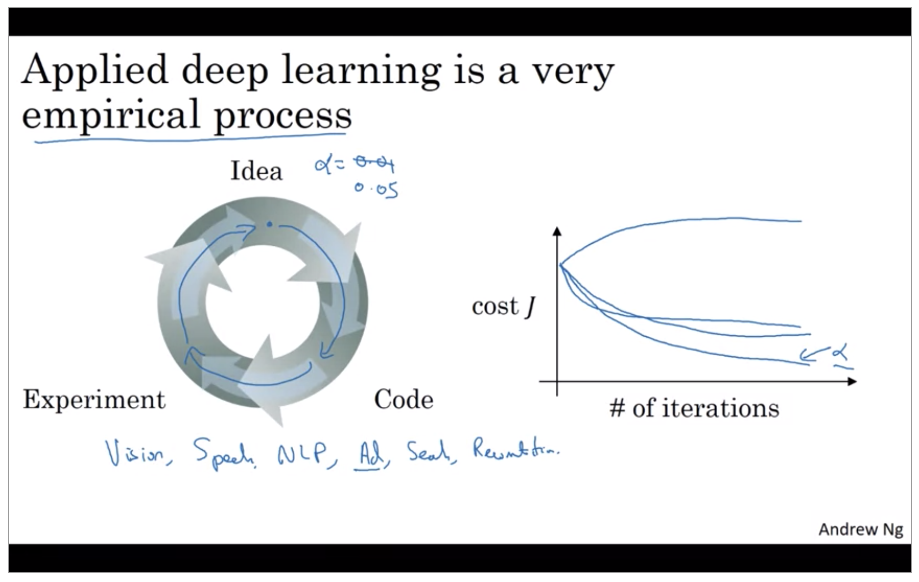
When you’re training a deep net for your own application you find that there may be a lot of possible settings for the hyper parameters that you need to just try out so apply deep learning today is a very empirical process where often you might have an idea for example you might have an idea for the best value for the learning rate you might say well maybe alpha equals 0.01 I want to try that then you implemented try it out and then see how that works and then based on that outcome you might say you know what I’ve changed online I want to increase the learning rate to 0.05 and so if you’re not sure what’s the best value for the learning ready-to-use you might try one value of the learning rate alpha and see their cost function j go down like this then you might try a larger value for the learning rate alpha and see the cost function blow up and diverge then you might try another version and see it go down really fast it’s inverse to higher value you might try another version and see it you know see the cost function J.
What does this have to do with the brain?
There is a very simplistic analogy between a single neuron in a neural network and a biological neuron-like that shown on the right, but I think that today even neuroscientists have almost no idea what even a single neuron is doing. A single neuron appears to be much more complex than we are able to characterize with neuroscience, and while some of what is doing is a little bit like logistic regression, there’s still a lot about what even a single neuron does that no human today understands.