DLS Course 2 - Week 1
Setting up your Machine Learning Application
Train / Dev / Test sets
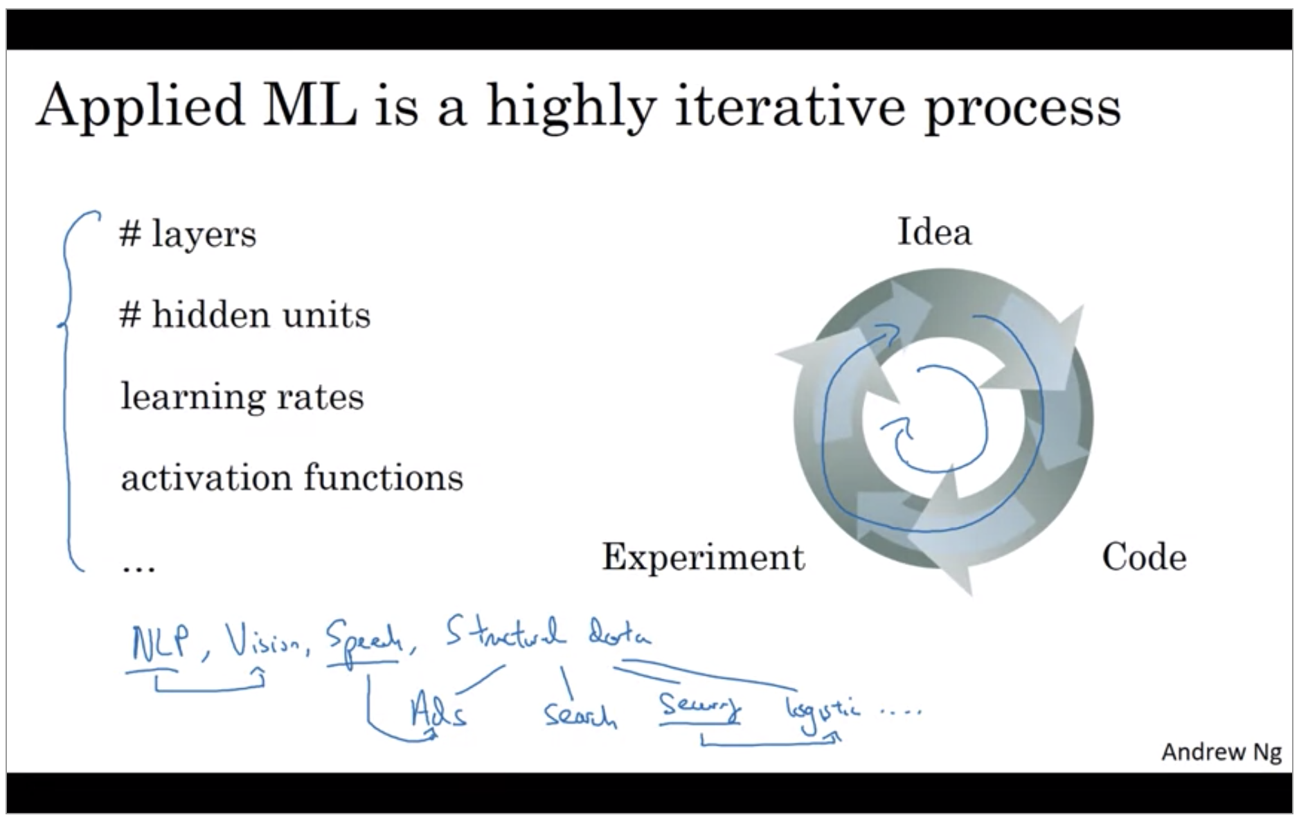
In practice applied machine learning is a highly iterative process, in which you often start with an idea, such as you want to build a neural network of a certain number of layers, certain number of hidden units, maybe on certain data sets and so on.
Even very experienced deep learning people find it almost impossible to correctly guess the best choice of hyper-parameters the very first time. And so today, applied deep learning is a very iterative process where you just have to go around this cycle many times to hopefully find a good choice of network for your application.
So one of the things that determine how quickly you can make progress is how efficiently you can go around this cycle. And setting up your data sets well in terms of your train, development and test sets can make you much more efficient at that.
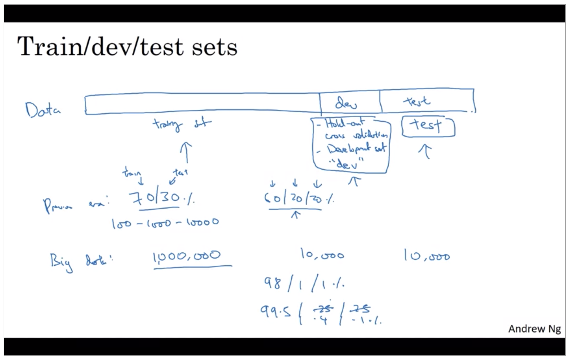
So in the previous era of machine learning, it was common practice to take all your data and split it according to maybe a 70/30% in terms of a people often talk about the 70/30 train test splits. If you have an explicit dev set or maybe a 60/20/20% split in terms of 60% train, 20% dev and 20% test. And several years ago this was widely considered best practice in machine learning. If you have maybe 100 examples in total, maybe 1000 examples in total, maybe after 10,000 examples. These sorts of ratios were perfectly reasonable rules of thumb.
But in the modern big data era, where, for example, you might have a million examples in total, then the trend is that your dev and test sets have been becoming a much smaller percentage of the total. The goal of the dev set or the development set is that you’re going to test different algorithms on it and see which algorithm works better. So the dev set just needs to be big enough for you to evaluate, say, two different algorithm choices or ten different algorithm choices and quickly decide which one is doing better. And you might not need a whole 20% of your data for that. If you need just 10,000 for your dev and 10,000 for your test, your ratio will be more like this 10,000 is 1% of 1 million so you’ll have 98% train, 1% dev, 1% test. And I’ve also seen applications where, if you have even more than a million examples, you might end up with 99.5% train and 0.25% dev, 0.25% test. Or maybe a 0.4% dev, 0.1% test.
One other trend we’re seeing in the era of modern deep learning is that more and more people train on mismatched train and test distributions.
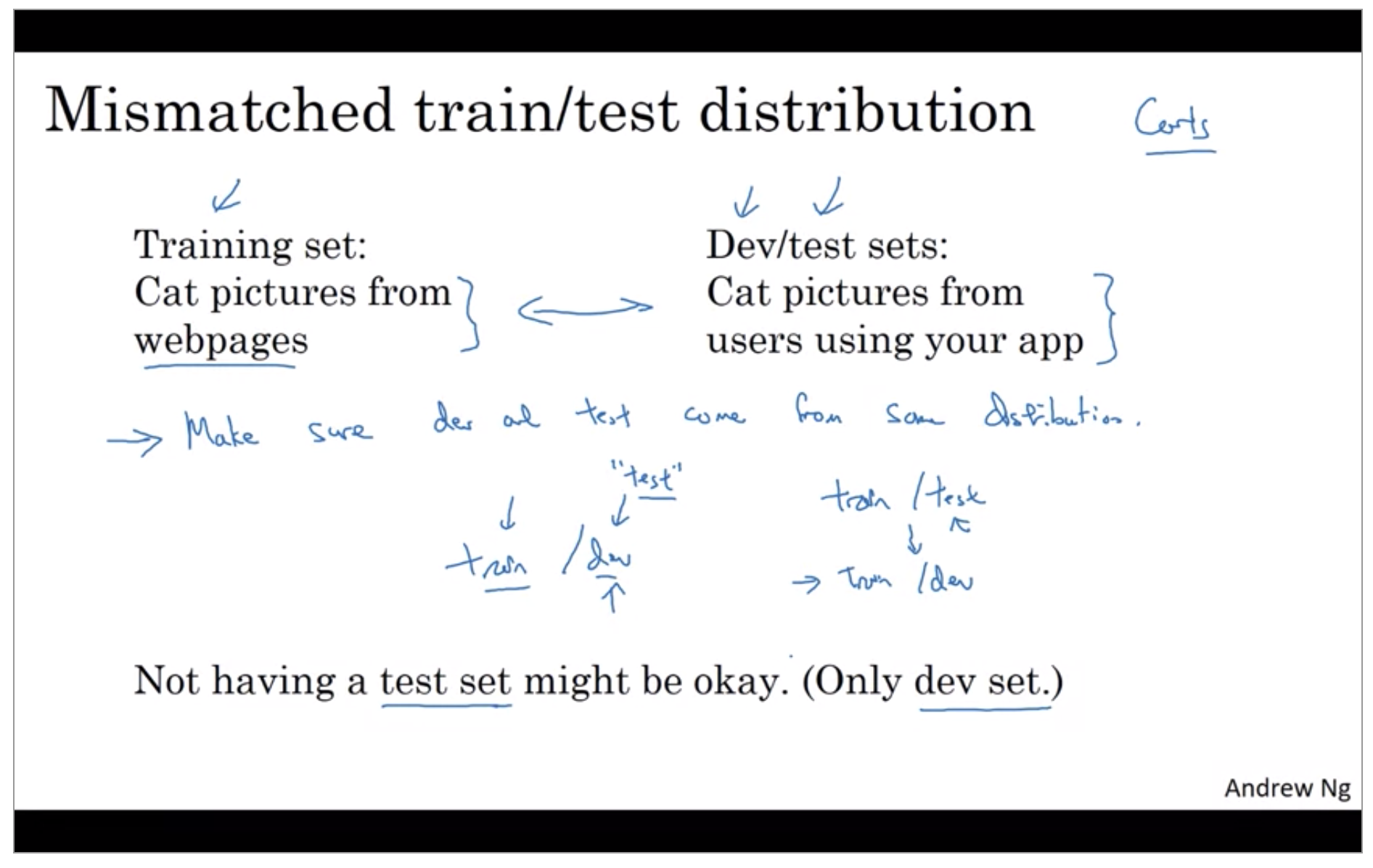
The rule of thumb I’d encourage you to follow in this case is to “Make sure that the dev and test sets come from the same distribution”.
Finally, it might be okay to not have a test set. Remember the goal of the test set is to give you a unbiased estimate of the performance of your final network, of the network that you selected. But if you don’t need that unbiased estimate, then it might be okay to not have a test set. So what you do, if you have only a dev set but not a test set, is you train on the training set and then you try different model architectures.
XXX: 아직 Dev(CV) set과 Test set을 차이를 이해하지 못하고 있음
Bias / Variance
I’ve noticed that almost all the really good machine learning practitioners tend to be very sophisticated in understanding of Bias and Variance. Bias and Variance is one of those concepts that’s easily learned but difficult to master. Even if you think you’ve seen the basic concepts of Bias and Variance, there’s often more new ones to it than you’d expect.
In the Deep Learning era, another trend is that there’s been less discussion of what’s called the bias-variance trade-off. You might have heard this thing called the bias-variance trade-off. But in Deep Learning era there’s less of a trade-off, so we’d still still solve the bias, we still solve the variance, but we just talk less about the bias-variance trade-off.
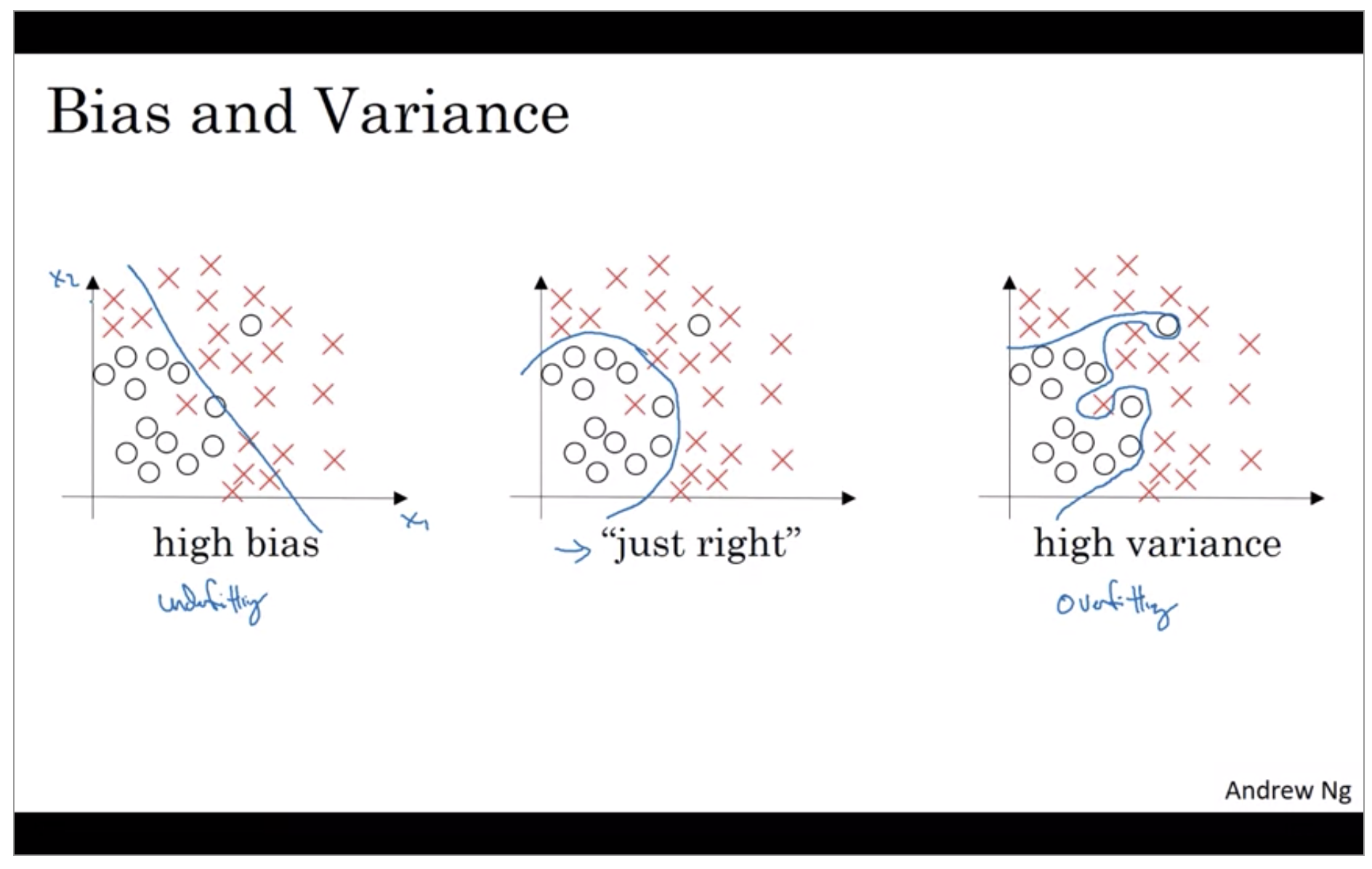
So in a 2D example like this, with just two features, X-1 and X-2, you can plot the data and visualize bias and variance. In high dimensional problems, you can’t plot the data and visualize division boundary. Instead, there are couple of different metrics, that we’ll look at, to try to understand bias and variance.
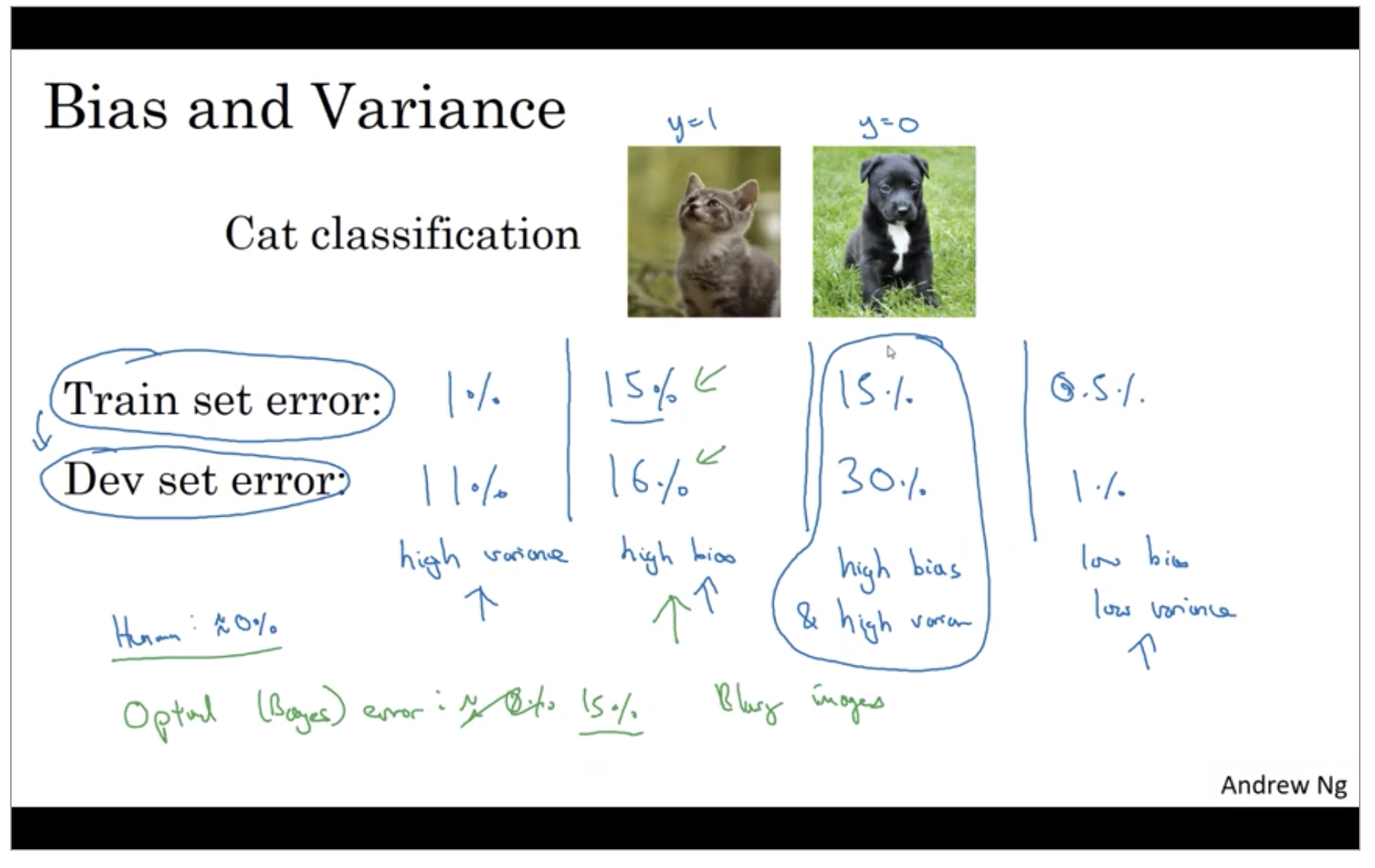
One subtlety is that this analysis is predicated on the assumption, that human level performance gets nearly 0% error or more generally, that the optimal error, sometimes called bayes error, so the bayes in optimal error is nearly 0%. It turns out that if the optimal error or the bayes error were much higher, say, it were 15%, then if you look at this classifier, 15% is actually perfectly reasonable for training set and you wouldn’t see it as high bias and also a pretty low variance.
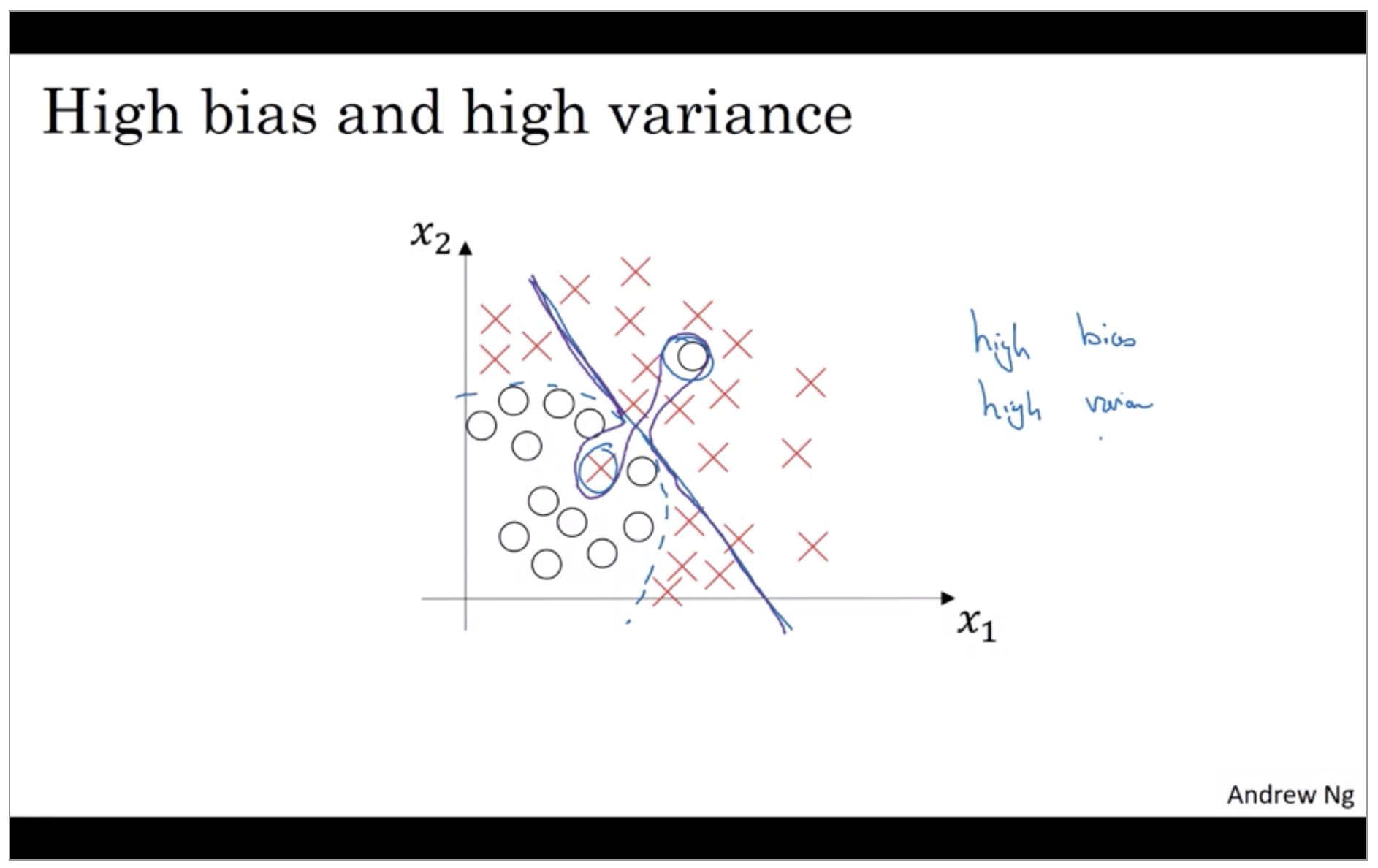
What does high bias and high variance looks like? This is kind of the worst of both worlds. Where it has high bias, because, by being a mostly linear classifier, is just not fitting. But by having too much flexibility in the middle, those two examples as well. And it has high variance, because it had too much flexibility to fit those two mislabel, or those live examples in the middle as well.
Well, this example is a little bit contrived in two dimensions, but with very high dimensional inputs. You actually do get things with high bias in some regions and high variance in some regions, and so it is possible to get classifiers like this in high dimensional inputs that seem less contrived.
Basic Recipe for Machine Learning
Fit the training set at least(reduce bias)
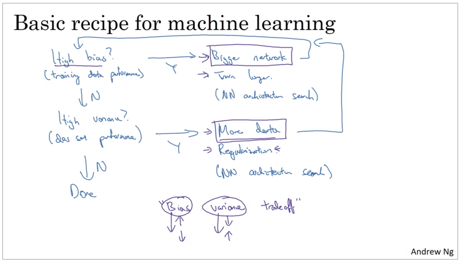
When training a neural network, here’s a basic recipe I will use. After having trained an initial model, I will first ask, does your algorithm have high bias? And so to try and evaluate if there is high bias, you should look at, really, the training set or the training data performance. And so, if it does have high bias, does not even fit in the training set that well, some things you could try would be to try pick a network, such as more hidden layers or more hidden units, or you could train it longer. Maybe run trains longer or try some more advanced optimization algorithms. Or you can also try, this is kind of a, maybe it work, maybe it won’t. There are a lot of different neural network architectures and maybe you can find a new network architecture that’s better suited for this problem. Putting this in parentheses because one of those things that, you just have to try. Maybe you can make it work, maybe not. Whereas getting a bigger network almost always helps. And training longer doesn’t always help, but it certainly never hurts.
So when training a learning algorithm, I would try these things until I can at least get rid of the bias problems, as in go back after I’ve tried this and keep doing that until I can fit, at least, fit the training set pretty well. If you have a big enough network, you should usually be able to fit the training data well so long as it’s a problem that is possible.
Then Do you have a variance problem?
Are you able to generalize from a pretty good training set performance to having a pretty good dev set performance? And if you have high variance, well, best way to solve a high variance problem is to get more data. Or you could try regularization to try to reduce overfitting. And then also, again, sometimes you just have to try it. But if you can find a more appropriate neural network architecture, sometimes that can reduce your variance problem as well, as well as reduce your bias problem.
But so I try these things and I kind of keep going back, until hopefully you find something with both low bias and low variance, whereupon you would be done.
So a couple of points to notice. First is that, depending on whether you have high bias or high variance, the set of things you should try could be quite different. So I’ll usually use the training dev set to try to diagnose if you have a bias or variance problem, and then use that to select the appropriate subset of things to try. So for example, if you actually have a high bias problem, getting more training data is actually not going to help. Or at least it’s not the most efficient thing to do. So being clear on how much of a bias problem or variance problem or both can help you focus on selecting the most useful things to try.
Second, in the earlier era of machine learning, there used to be a lot of discussion on what is called the bias variance tradeoff. And the reason for that was that, for a lot of the things you could try, you could increase bias and reduce variance, or reduce bias and increase variance. But back in the pre-deep learning era, we didn’t have many tools, we didn’t have as many tools that just reduce bias or that just reduce variance without hurting the other one. But in the modern deep learning, big data era, so long as you can keep training a bigger network, and so long as you can keep getting more data, which isn’t always the case for either of these, but if that’s the case, then getting a bigger network almost always just reduces your bias without necessarily hurting your variance, so long as you regularize appropriately. And getting more data pretty much always reduces your variance and doesn’t hurt your bias much.
Regularizing your neural network
If you suspect your neural network is over fitting your data. That is you have a high variance problem, one of the first things you should try per probably regularization. The other way to address high variance, is to get more training data that’s also quite reliable. But you can’t always get more training data, or it could be expensive to get more data.
\[\min_{w,b}j(w,b), w \in \R^{n_x}, b \in \R \\ J(w,b) = \frac{1}{m}\sum_{i=1}^m L(\hat{y}^{(i)}, y^{(i)}) + \frac{\lambda}{2m} \left\lVert w \right\rVert^2_2 \\ \left\lVert w \right\rVert^2_2 = \sum_{j=1}^{n_x} w_j^2 = w^Tw\]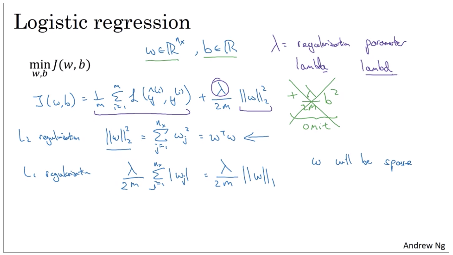
Now, why do you regularize just the parameter w? Why don’t we add something here about b as well? In practice, you could do this, but I usually just omit this. Because if you look at your parameters, w is usually a pretty high dimensional parameter vector, especially with a high variance problem. Maybe w just has a lot of parameters, so you aren’t fitting all the parameters well, whereas b is just a single number.
So L2 regularization is the most common type of regularization. You might have also heard of some people talk about L1 regularization. And that’s when you add, instead of this L2 norm, you instead add a term that is lambda/m of sum over of this.
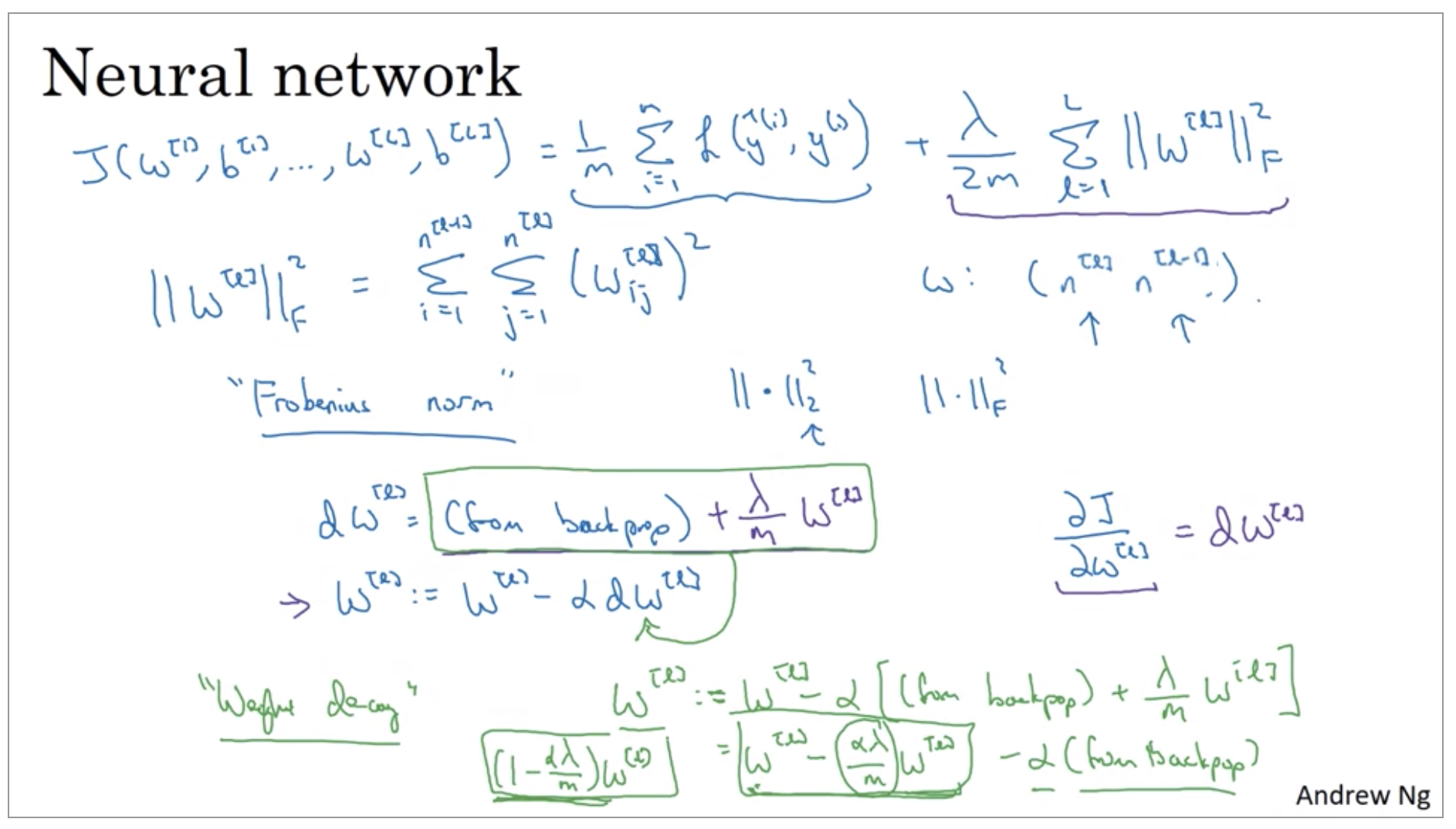
Frobenius norm: https://en.wikipedia.org/wiki/Matrix_norm#Frobenius_norm
Why regularization reduces overfitting?
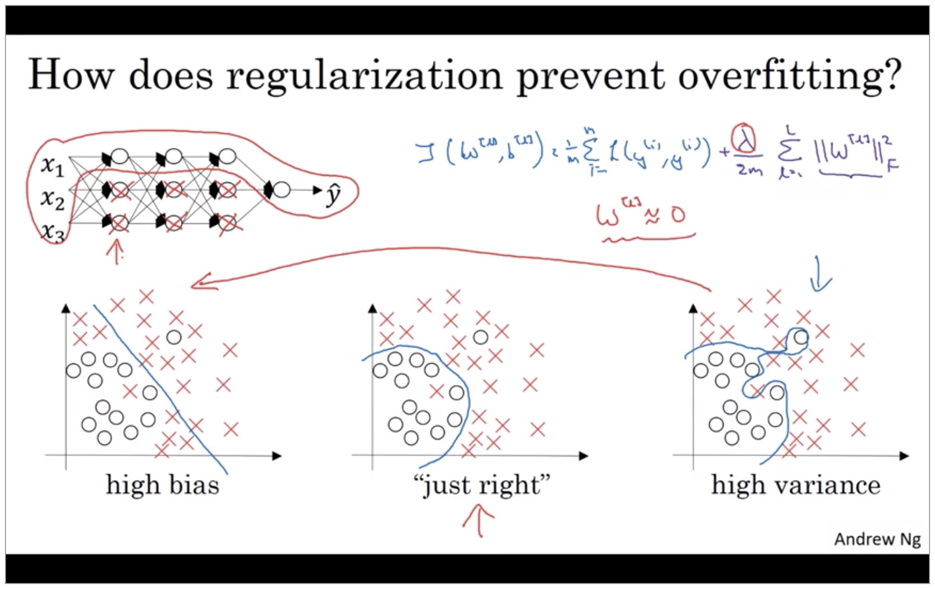
One piece of intuition is that if you crank regularization lambda to be really, really big, they’ll be really incentivized to set the weight matrices W to be reasonably close to zero.
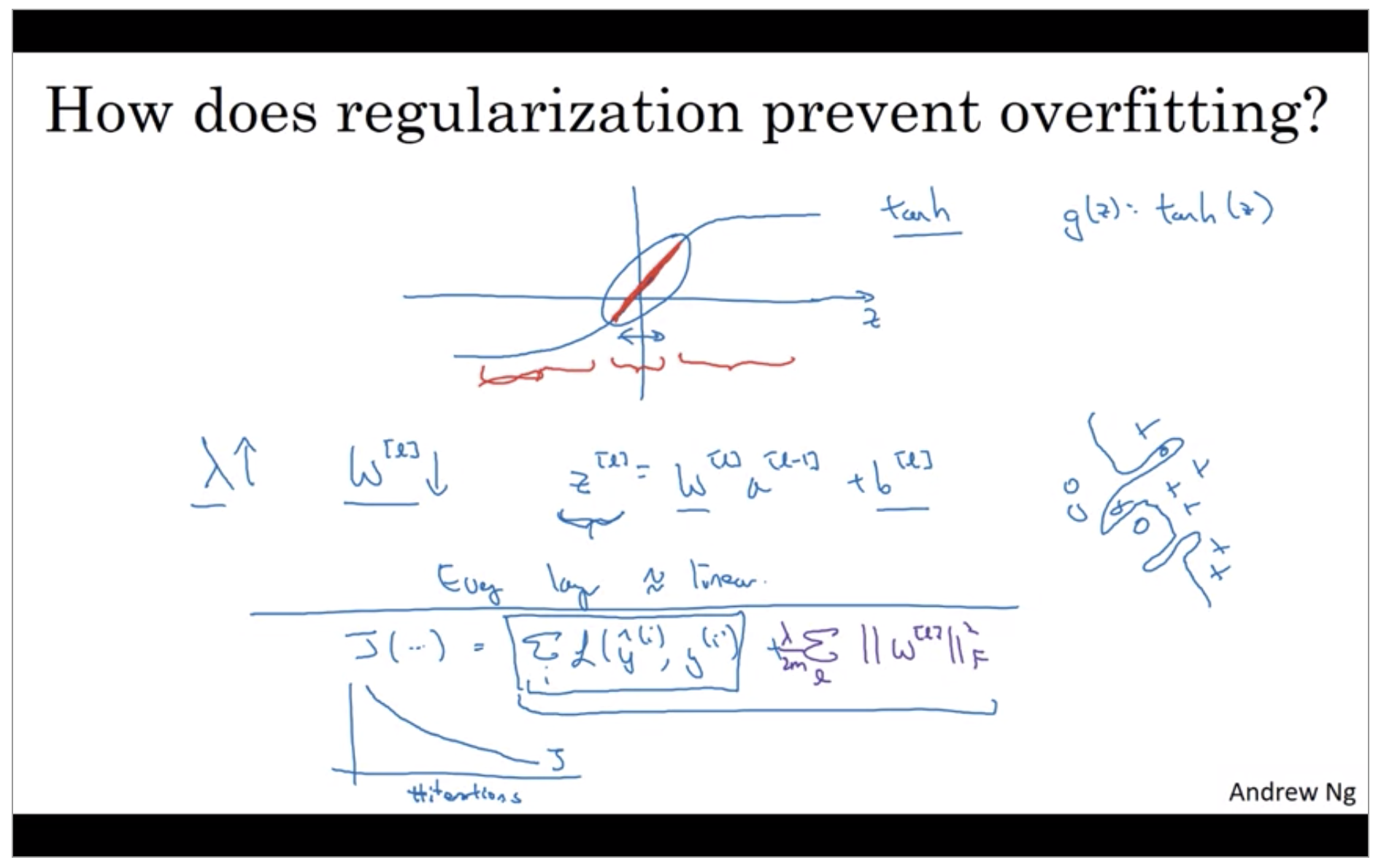
If the regularization parameters are very large, the parameters W are very small, so Z will be relatively small, kind of ignoring the effects of b for now. so Z will be relatively small or, really, it takes on a small range of values. And so the activation function if is tanh, say, will be relatively linear. And so your whole neural network will be computing something not too far from a big linear function which is therefore pretty simple function rather than a very complex highly non-linear function.
So to debug gradient descent make sure that you’re plotting this new definition of J that includes this second term as well. Otherwise you might not see J decrease monotonically on every single iteration.
Dropout Regularization
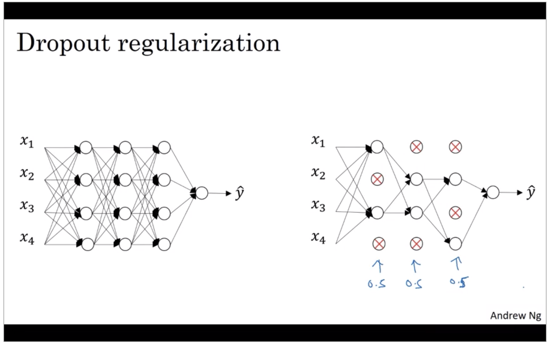
Another very powerful regularization techniques is called “dropout”. Let’s say you train a neural network like the one on the left and there’s over-fitting. Let’s say that for each of these layers, we’re going to for each node, toss a coin and have a 0.5 chance of keeping each node and 0.5 chance of removing each node. So, after the coin tosses, maybe we’ll decide to eliminate those nodes, then what you do is actually remove all the ingoing and outgoing things from that no as well. So you end up with a much smaller, really much diminished network.
So, maybe it seems like a slightly crazy technique. They just go around coding those are random, but this actually works. But you can imagine that because you’re training a much smaller network on each example or maybe just give a sense for why you end up able to regularize the network, because these much smaller networks are being trained.
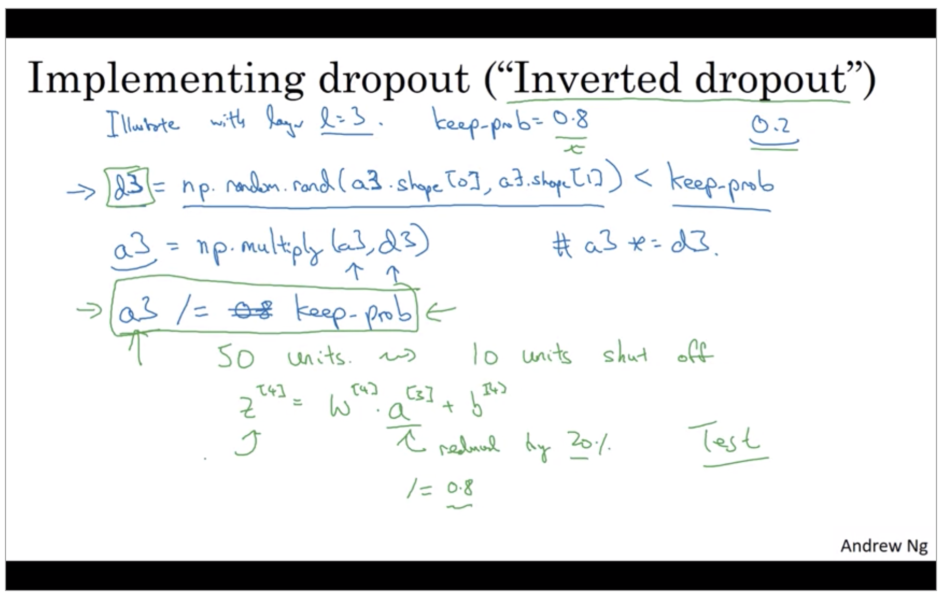
And there was a 20% chance of each of the elements being zero, just multiply operation ends up zeroing out, the corresponding element of d3. If you do this in python, technically d3 will be a boolean array where value is true and false, rather than one and zero. But the multiply operation works and will interpret the true and false values as one and zero.
This inverted dropout technique by dividing by the keep.prob, it ensures that the expected value of a3 remains the same. And it turns out that at test time, when you trying to evaluate a neural network, which we’ll talk about on the next slide, this inverted dropout technique, there is there is line to are due to the green box at dropping out. This makes test time easier because you have less of a scaling problem.
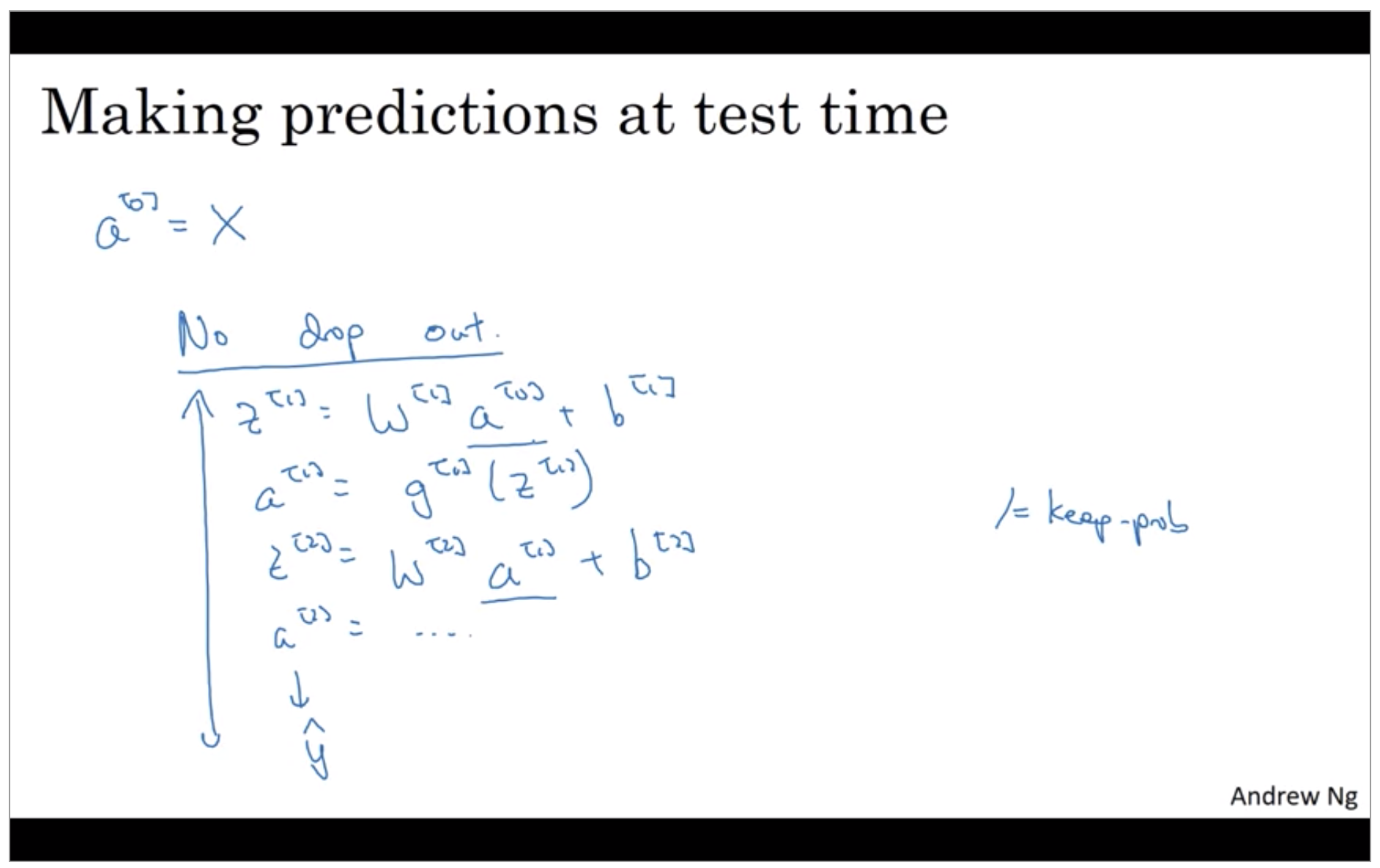
But notice that the test time you’re not using dropout explicitly and you’re not tossing coins at random, you’re not flipping coins to decide which hidden units to eliminate. And that’s because when you are making predictions at the test time, you don’t really want your output to be random. If you are implementing dropout at test time, that just add noise to your predictions.
Understanding Dropout
Drop out does this seemingly crazy thing of randomly knocking out units on your network. Why does it work so well with a regularizer?
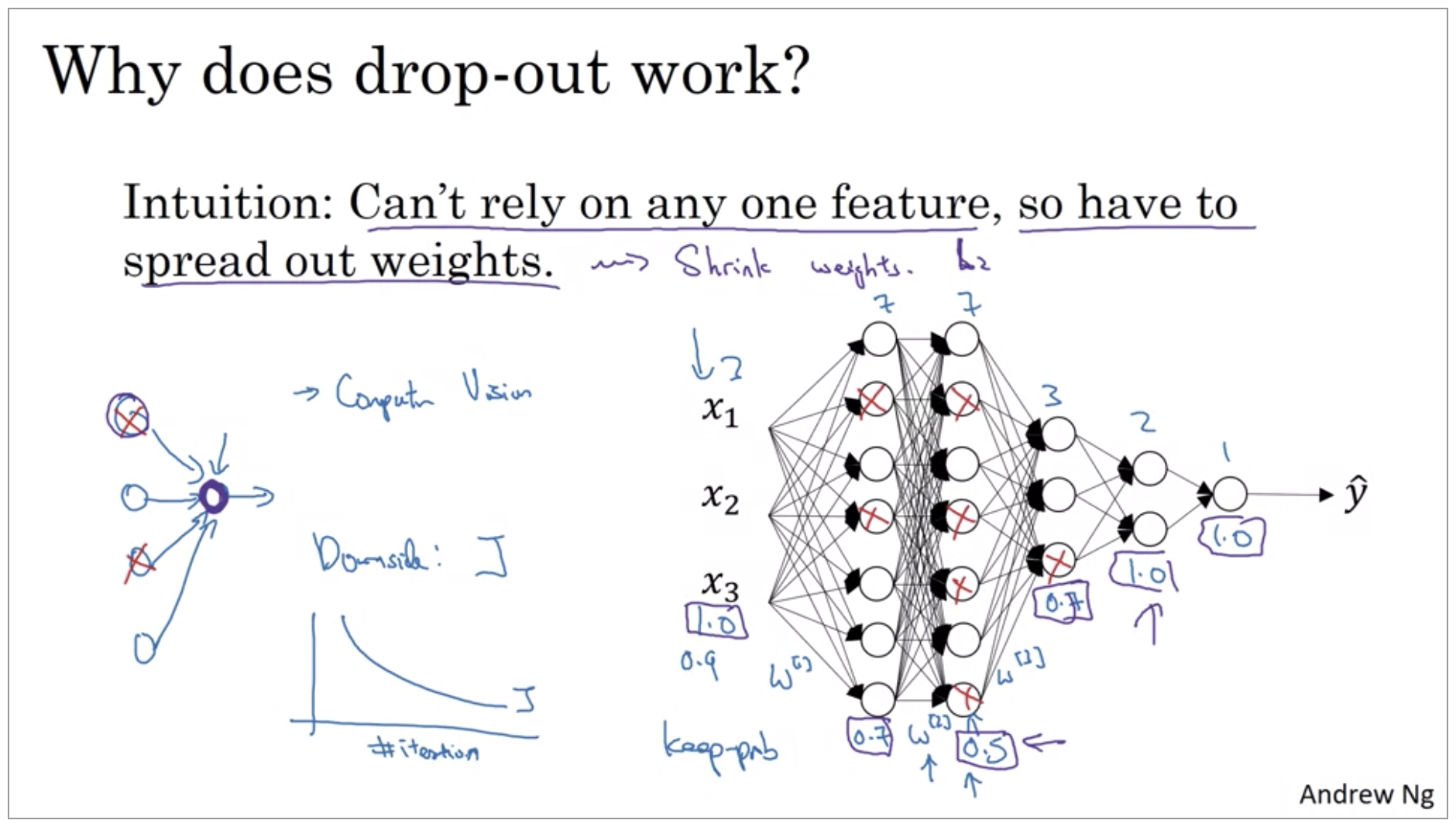
Many of the first successful implementations of drop outs were to computer vision. So in computer vision, the input size is so big, inputting all these pixels that you almost never have enough data. And so drop out is very frequently used by computer vision. And there’s some computer vision researchers that pretty much always use it, almost as a default. And there’s some computer vision researchers that pretty much always use it, almost as a default. But really the thing to remember is that drop out is a regularization technique, it helps prevent over-fitting. And so, unless my algorithm is over-fitting, I wouldn’t actually bother to use drop out. So it’s used somewhat less often than other application areas. There’s just with computer vision, you usually just don’t have enough data, so you’re almost always overfitting, which is why there tends to be some computer vision researchers who swear by drop out. But their intuition doesn’t always generalize I think to other disciplines.
One big downside of drop out is that the cost function J is no longer well-defined. On every iteration, you are randomly killing off a bunch of nodes. And so, if you are double checking the performance of grade and dissent, it’s actually harder to double check that you have a well defined cost function J that is going downhill on every iteration. Because the cost function J that you’re optimizing is actually less. Less well defined, or is certainly hard to calculate. So you lose this debugging tool to will a plot, a graph like this. So what I usually do is turn off drop out, you will set key prop equals one, and I run my code and make sure that it is monotonically decreasing J, and then turn on drop out and hope that I didn’t introduce bugs into my code during drop out.
Other regularization methods
In addition to L2 regularization and drop out regularization there are few other techniques to reducing over fitting in your neural network.
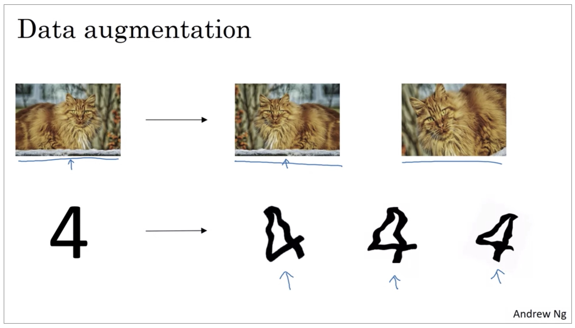
If you are over fitting getting more training data can help, but getting more training data can be expensive and sometimes you just can’t get more data. But what you can do is augment your training set by taking image like this. So data augmentation can be used as a regularization technique, in fact similar to regularization.
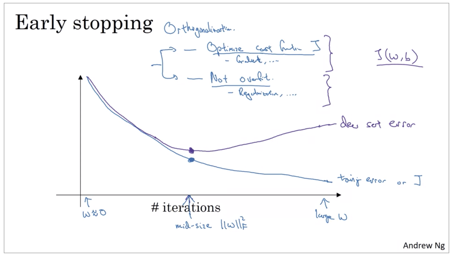
There’s one other technique that is often used called early stopping. So what early stopping does is, you will say well, it looks like your neural network was doing best around that iteration, so we just want to stop trading on your neural network halfway and take whatever value achieved this dev set error. So why does this work? Well when you’ve haven’t run many iterations for your neural network yet your parameters w will be close to zero. Because with random initialization you probably initialize w to small random values so before you train for a long time, w is still quite small. And as you iterate, as you train, w will get bigger and bigger and bigger until here maybe you have a much larger value of the parameters w for your neural network. So what early stopping does is by stopping halfway you have only a mid-size rate w. And so similar to L2 regularization by picking a neural network with smaller norm for your parameters w, hopefully your neural network is over fitting less.
But, to me the main downside of early stopping is that this couples these two tasks. So you no longer can work on these two problems independently, because by stopping gradient decent early, you’re sort of breaking whatever you’re doing to optimize cost function J,because now you’re not doing a great job reducing the cost function J. You’ve sort of not done that that well. And then you also simultaneously trying to not over fit. So instead of using different tools to solve the two problems, you’re using one that kind of mixes the two. And this just makes the set of things you could try are more complicated to think about.
Rather than using early stopping, one alternative is just use L2 regularization then you can just train the neural network as long as possible. I find that this makes the search space of hyper parameters easier to decompose, and easier to search over. But the downside of this though is that you might have to try a lot of values of the regularization parameter lambda.
Setting up your optimization problem
Normalizing inputs
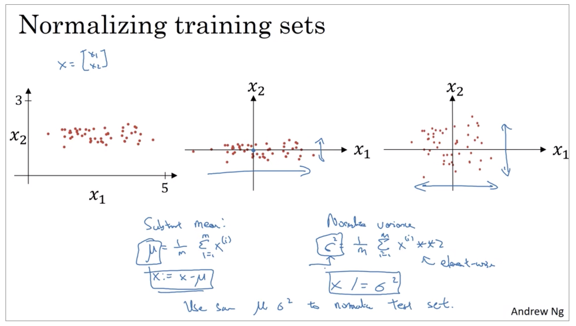
If you use this to scale your training data, then use the same mu and sigma squared to normalize your test set, right? In particular, you don’t want to normalize the training set and the test set differently. Whatever this value is and whatever this value is, use them in these two formulas so that you scale your test set in exactly the same way, rather than estimating mu and sigma squared separately on your training set and test set. Because you want your data, both training and test examples, to go through the same transformation defined by the same mu and sigma squared calculated on your training data.
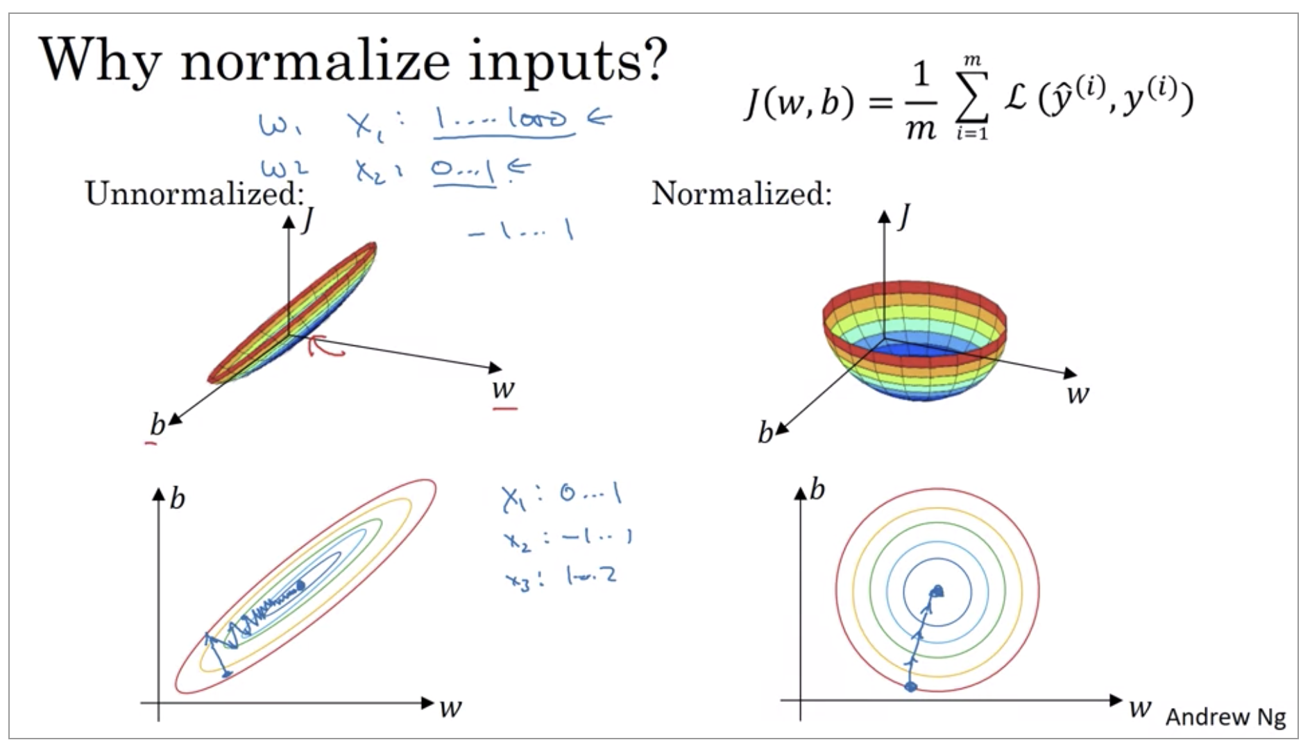
Why do we want to normalize the input features? If your features are on very different scales, say the feature X1 ranges from 1 to 1,000, and the feature X2 ranges from 0 to 1, then it turns out that the ratio or the range of values for the parameters w1 and w2 will end up taking on very different values. And so maybe these axes should be w1 and w2, but I’ll plot w and b, then your cost function can be a very elongated bowl like that.
Whereas if you normalize the features, then your cost function will on average look more symmetric. And if you’re running gradient descent on the cost function like the one on the left, then you might have to use a very small learning rate because if you’re here that gradient descent might need a lot of steps to oscillate back and forth before it finally finds its way to the minimum. Whereas if you have a more spherical contours, then wherever you start gradient descent can pretty much go straight to the minimum. You can take much larger steps with gradient descent rather than needing to oscillate around like like the picture on the left.
Vanishing / Exploding gradients
One of the problems of training neural network, especially very deep neural networks, is data vanishing and exploding gradients.What that means is that when you’re training a very deep network your derivatives or your slopes can sometimes get either very, very big or very, very small, maybe even exponentially small, and this makes training difficult.
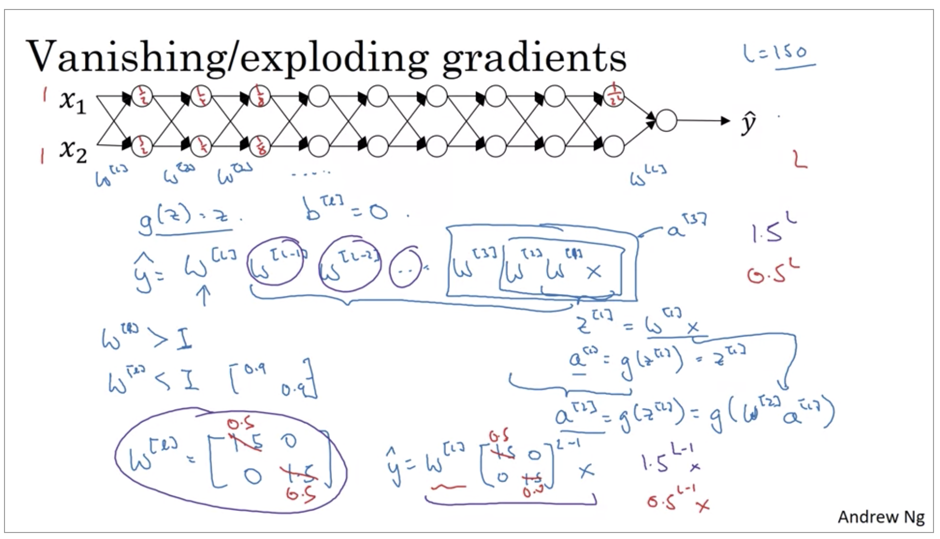
So the intuition I hope you can take away from this is that at the weights W, if they’re all just a little bit bigger than one or just a little bit bigger than the identity matrix, then with a very deep network the activations can explode. And if W is just a little bit less than identity. So this maybe here’s 0.9, 0.9, then you have a very deep network, the activations will decrease exponentially.
With some of the modern neural networks, L equals 150. Microsoft recently got great results with 152 layer neural network. But with such a deep neural network, if your activations or gradients increase or decrease exponentially as a function of L, then these values could get really big or really small.
Weight Initialization for Deep Networks
Very deep neural networks can have the problems of vanishing and exploding gradients. It turns out that a partial solution to this, doesn’t solve it entirely but helps a lot, is better or more careful choice of the random initialization for your neural network.
-
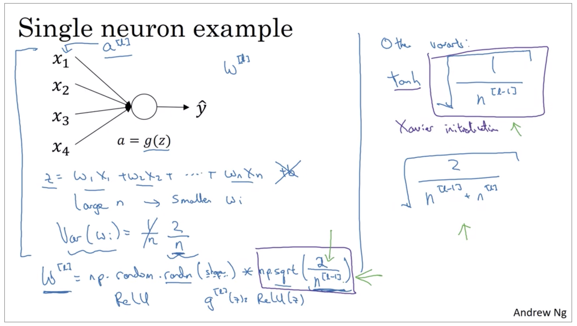
For ReLu: He(He-et-al) initialization
\[np.random.randn(shape) * \sqrt{\frac{2}{n^{[l-1]}}}\] -
For tanh: Xavier initialization
\[np.random.randn(shape) * \sqrt{\frac{2}{n^{[l-1]} + n^{[l]}}}\]https://medium.com/@prateekvishnu/xavier-and-he-normal-he-et-al-initialization-8e3d7a087528
Numerical approximation of gradients
When you implement back propagation you’ll find that there’s a test called creating checking that can really help you make sure that your implementation of back prop is correct.
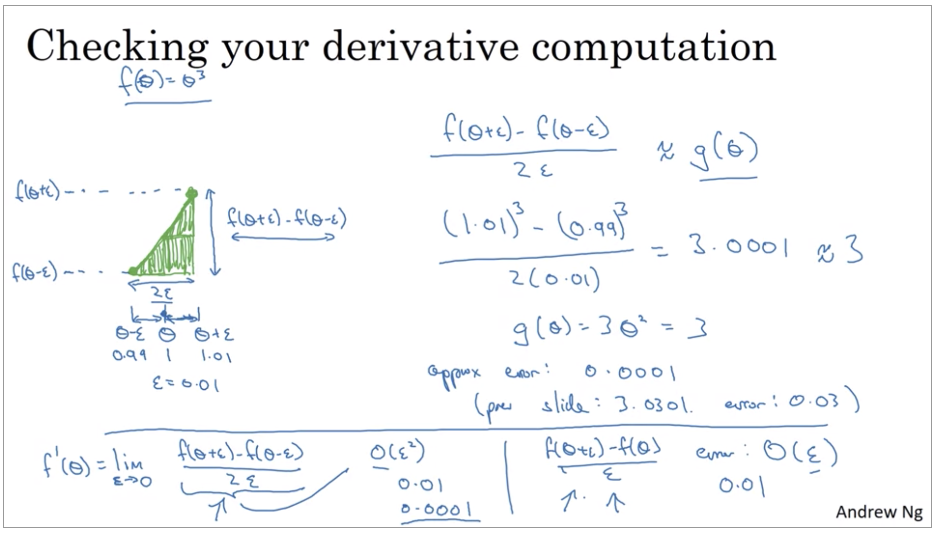
This two sided difference way of approximating the derivative you find that this is extremely close to 3. And so this gives you a much greater confidence that g of theta is probably a correct implementation of the derivative of F. When you use this method for gradient checking and back propagation, this turns out to run twice as slow as you were to use a one-sided difference. It turns out that in practice I think it’s worth it to use this other method because it’s just much more accurate.
Gradient checking
Gradient checking is a technique that’s helped me save tons of time, and helped me find bugs in my implementations of back propagation many times.
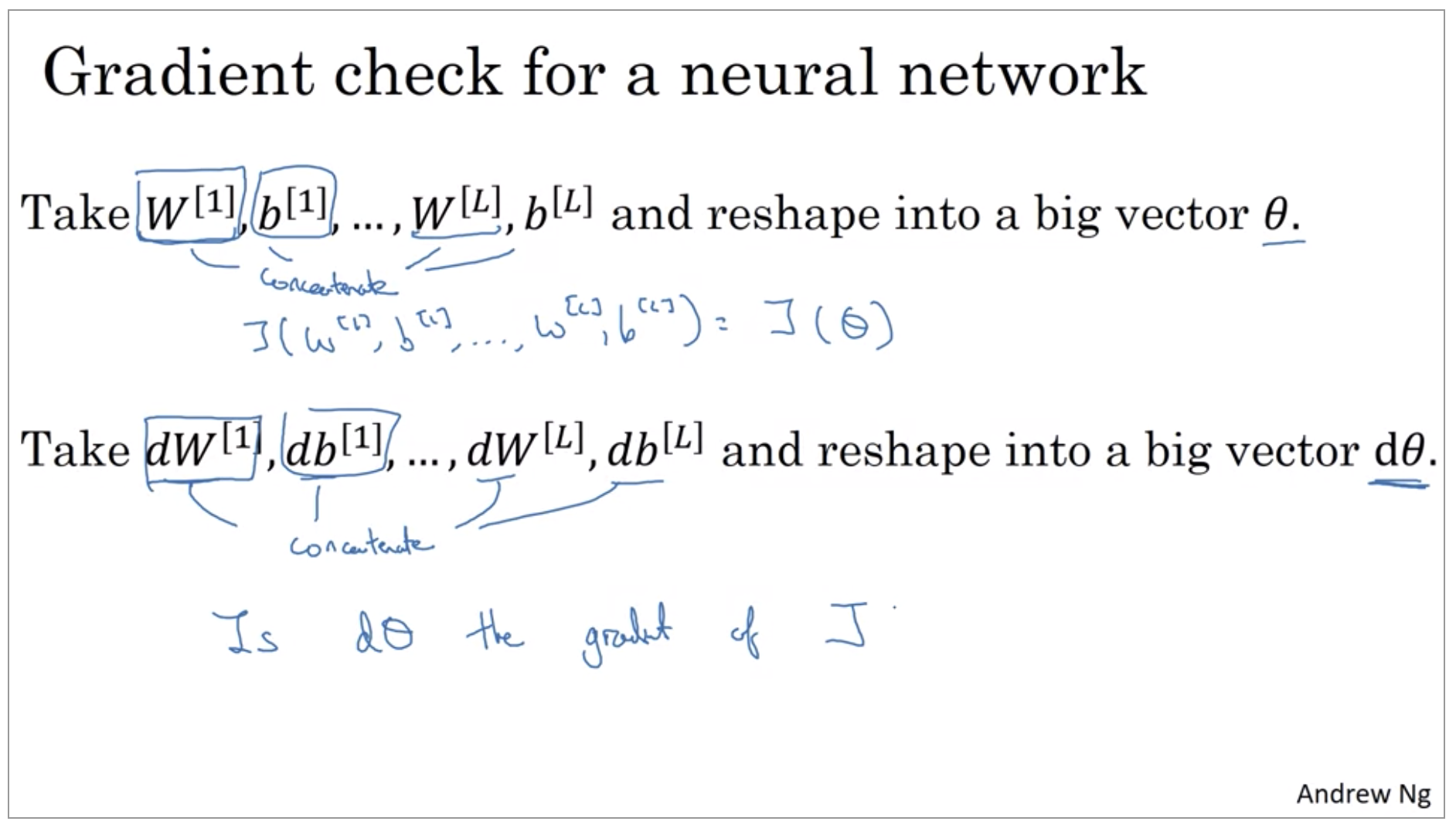
The sort of reshaping and concatenation operation, you can then reshape all of these derivatives into a giant vector theta and d theta. You can then reshape all of these derivatives into a giant vector d theta which has the same dimension as theta. So the question is, now, is d theta the gradient of the slope of the cost function J?
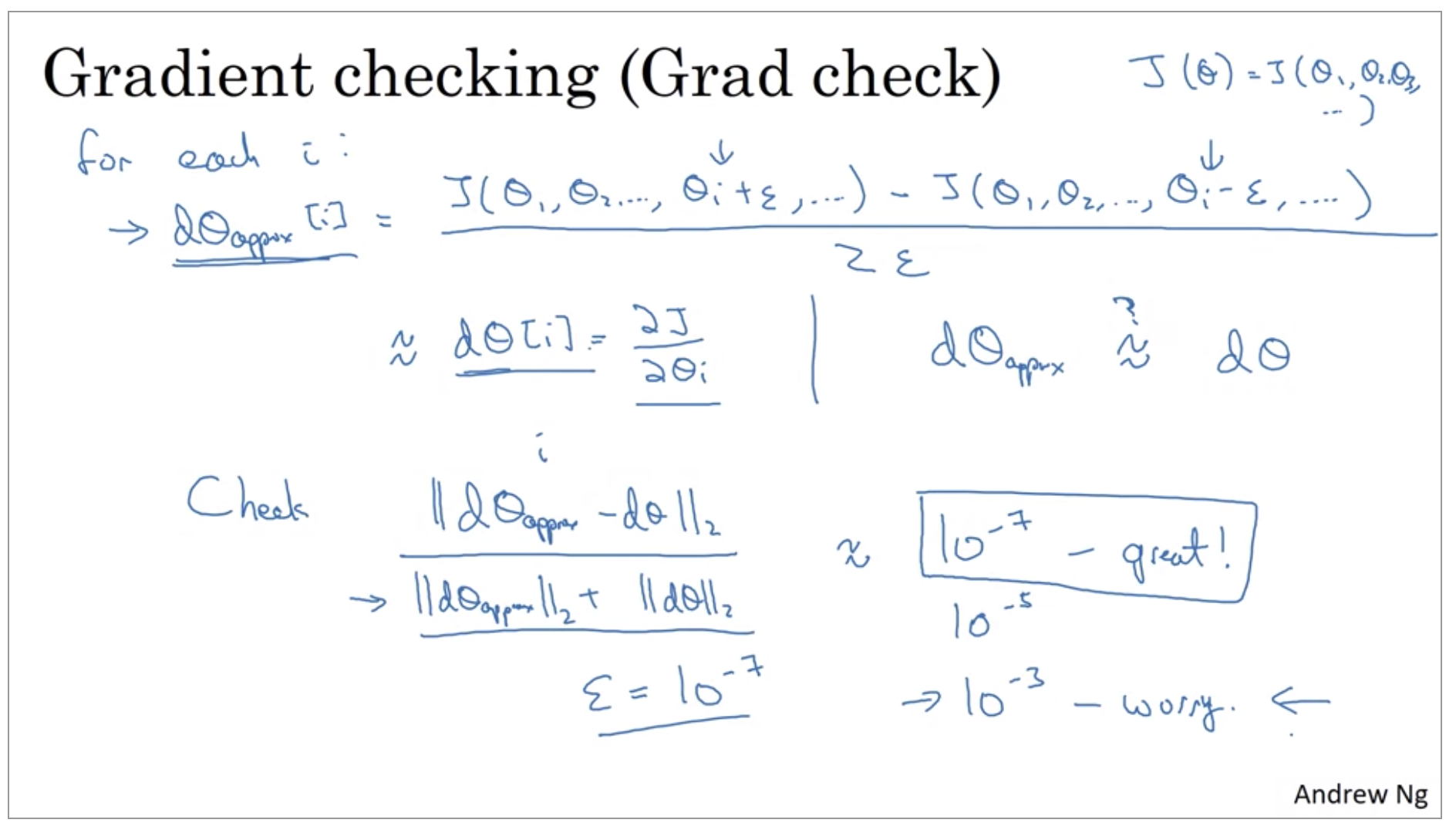
I would compute the euclidean distance between these two vectors, d theta approx minus d theta, so just the l2 norm of this.
So we implement this in practice, I use epsilon equals maybe 10 to the minus 7, so minus 7. And with this range of epsilon, if you find that this formula gives you a value like 10 to the minus 7 or smaller, then that’s great. It means that your derivative approximation is very likely correct. This is just a very small value. If it’s maybe on the range of 10 to the -5, I would take a careful look. Maybe this is okay. But I might double-check the components of this vector, and make sure that none of the components are too large. And if some of the components of this difference are very large, then maybe you have a bug somewhere. If any bigger than 10 to minus 3, then I would be quite concerned. I would be seriously worried about whether or not be a bug.
Gradient Checking Implementation Notes
I want to share with you some practical tips or some notes on how to actually go about implementing this for your neural network.
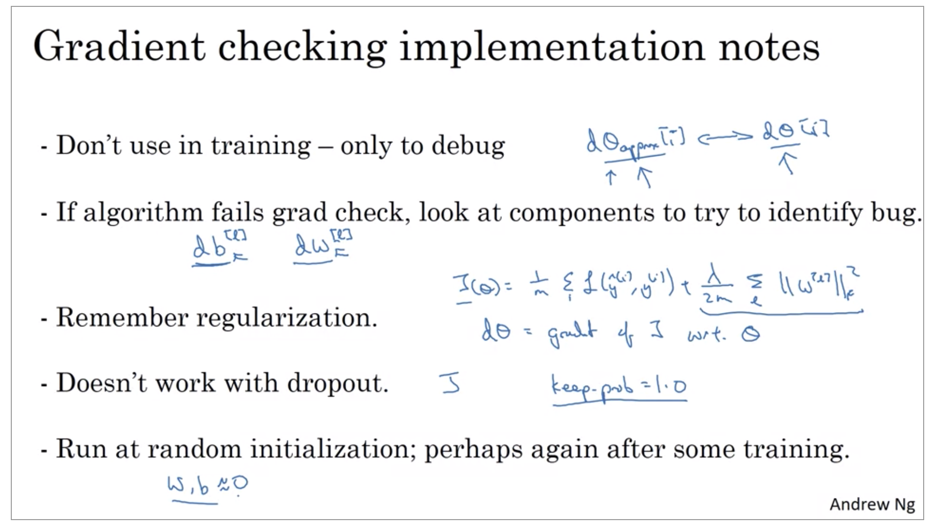
First, don’t use grad check in training, only to debug. So what I mean is that, computing d theta approx i, for all the values of i, this is a very slow computation.
Second, if an algorithm fails grad check, look at the components, look at the individual components, and try to identify the bug. So what I mean by that is if d theta approx is very far from d theta, what I would do is look at the different values of i to see which are the values of d theta approx that are really very different than the values of d theta.
Next, when doing grad check, remember your regularization term if you’re using regularization. So if your cost function is J of theta equals 1 over m sum of your losses and then plus this regularization term.
And you should have that d theta is gradient of J with respect to theta, including this regularization term. So just remember to include that term.
Next, grad check doesn’t work with dropout, because in every iteration, dropout is randomly eliminating different subsets of the hidden units. There isn’t an easy to compute cost function J that dropout is doing gradient descent on. It turns out that dropout can be viewed as optimizing some cost function J, but it’s cost function J defined by summing over all exponentially large subsets of nodes they could eliminate in any iteration. So the cost function J is very difficult to compute, and you’re just sampling the cost function every time you eliminate different random subsets in those we use dropout. So it’s difficult to use grad check to double check your computation with dropouts. So what I usually do is implement grad check without dropout. And then turn on dropout and hope that my implementation of dropout was correct.
And one thing you could do is run grad check at random initialization and then train the network for a while so that w and b have some time to wander away from 0, from your small random initial values. And then run grad check again after you’ve trained for some number of iterations.